Market Risk: Standard Deviation
Dollar Standard Deviation
In risk management, when we talk about the standard deviation of a security, we are almost always talking about the standard deviation of the returns for that security. While this is almost always the case, there will be times when we want to express standard deviation and other risk parameters in terms of dollars (or euros, yen, etc.).
In order to calculate the expected dollar standard deviation of a security, we begin by calculating the expected return standard deviation, and then multiply this value by the current dollar value of the security (or, in the case of futures, the nominal value of the contract). It’s that simple. If we have 200 worth of ABC stock, and the stock’s return standard deviation is 3%, then the expected dollar standard deviation is 3% × 200 = 6.
What you should not do is calculate the dollar standard deviation directly from past dollar returns or price changes. The difference is subtle, and it is easy to get confused. The reason that we want to calculate the return standard deviation first is that percentage returns are stable over time, whereas dollar returns rarely are. This may not be obvious in the short term, but consider what can happen to a security over a long period of time. Take, for example, IBM. In 1963, the average split-adjusted closing price of IBM was 2.00, compared to 127.53 in 2010.
Even though the share price of IBM grew substantially over those 47 years, the daily return standard deviation was relatively stable, 1.00% in 1963 versus 1.12% in 2010.
Annualization
Up until now, we have not said anything about the frequency of returns. Most of the examples have made use of daily data. Daily returns are widely available for many financial assets, and daily return series often serve as the starting point for risk management models. That said, in has become common practice in finance and risk management to present standard deviation as an annual number.
For example, if somebody tells you that the option-implied standard deviation of a Microsoft one-month at-the-money call option is 18%—unless they specifically tell you otherwise—this will almost always mean that the annualized standard deviation is 18%.
It doesn’t matter that the option has one month to expiration, or that the model used to calculate the implied standard deviation used daily returns; the standard deviation quoted is annualized.
Square-root rule for I.I.D.s
If the returns of a security meet certain requirements, namely that the returns are independently and identically distributed, converting a daily standard deviation to an annual standard deviation is simply a matter of multiplying by the square root of days in the year.
For example, if we estimate the standard deviation of daily returns as 2.00%, and there are 256 business days in a year, then the expected standard deviation of annual returns is simply $32 \% = 2 \% \times \sqrt{256}$.
If we have a set of non-overlapping weekly returns, we could calculate the standard deviation of weekly returns and multiply by the square root of 52 to get the expected standard deviation of annual returns. This square-root rule only works if returns are i.i.d.
Non I.I.D Case
If the distribution of returns is changing over time, as with our GARCH model, or returns display serial correlation, which is not uncommon, then the standard deviation of annual returns could be higher or lower than the square-root rule would predict.
If returns are not i.i.d. and we are really interested in trying to predict the expected standard deviation of annual returns, then we should not use the square-root rule. We need to use a more sophisticated statistical model, or use actual annual returns as the basis of our calculation.
That said, in many settings, such as quoting option-implied standard deviation or describing the daily risk of portfolio returns, annualization is mostly about presentation, and making comparison of statistics easier. In these situation, we often use the square root rule, even when returns are not i.i.d. In these settings, doing anything else would actually cause more confusion. As always, if you are unsure of the convention, it is best to clearly explain how you arrived at your calculation.
Market Risk: Value At Risk
Defined as Losses or Returns
VaR was popularized by J.P. Morgan in the 1990s. The executives at J.P. Morgan wanted their risk managers to generate one statistic that summarized the risk of the firm’s entire portfolio, at the end of each day. What they came up with was VaR.
In order to formally define VaR, we begin by defining a random variable L, which represents the loss to our portfolio. L is simply the opposite of the return to our portfolio. If the return of our portfolio is −600, then the loss, L, is +600. For a given confidence level, $\gamma$, then, value at risk is defined as
\[P[L\geq VaR_{\gamma}]=1-\gamma\]We can also define VaR directly in terms of returns. If we multiply both sides of the inequality in the preceding equation by −1, and replace −L with R, we come up with
\[P[L\leq -VaR_{\gamma}]=1-\gamma\]While these two equations are equivalent, defining VaR in terms of losses is more common. It has the advantage that, for most portfolios for reasonable confidence levels, VaR will almost always be a positive number.
In practice, rather than saying that your VaR is 400, it is often best to resolve any ambiguity by stating that your VaR is a loss of 400.
Advantages of VaR as a Risk Measure
One of the primary appeals of VaR is its simplicity. The concept of VaR is intuitive, even to those not versed in statistics. Because it boils risk down to a single number, VaR also provides us with a convenient way to track the risk of a portfolio over time.
Another appealing feature of VaR is that is focuses on losses. This may seem like an obvious criterion for a risk measure, but variance and standard deviation treat positive and negative deviations from the mean equally. For many risk managers, VaR also seems to strike the right balance, by focusing on losses that are significant, but not too extreme. We’ll have more to say about this at the end of the chapter, when we discuss backtesting.
VaR also allows us to aggregate risk across a portfolio with many different types of securities (e.g., stocks, bonds, futures, options, etc.). Prior to VaR, risk managers were often forced to evaluate different segments of a portfolio separately. For example, for the bonds in a port- folio they may have looked at the interest rate sensitivities, and for the equities they may have looked at how much exposure there was to different industries.
Finally, VaR is robust to outliers. As is true of the median or any quantile measure, a {: .align-center}single large event in our data set (or the absence of one) will usually not change our estimate of VaR. This advantage of VaR is a direct consequence of one of its deepest flaws, that it ignores the tail of the distribution. As we will see in the next chapter, expected shortfall, a closely related measure, has exactly the opposite problem: It incorporates the tail of the distribution, but it is not robust to outliers.
Delta-Normal VaR
One of the simplest and easiest ways to calculate VaR is to make what are known as delta-normal assumptions. For any underlying asset, we assume that the log returns are normally distributed and we approximate the returns of any option using its delta-adjusted exposure. The delta-normal model includes additional assumptions when multiple securities are involved, which we will cover when we begin to look at portfolio risk measures.
To calculate the delta-normal VaR of a security, we start by calculating the standard deviation of returns for the security or, in the case of an option, for the returns of the option’s underlying security.
For regular securities, we then multiply the return standard deviation by the absolute market value or notional of our position to get the position’s standard deviation. For options we multiply by the absolute delta-adjusted exposure. The delta adjusted exposure of a single option being the underlying security’s price multiplied by the option’s delta.
For Black-Scholes model, the standard return has the following distribution:
\[\frac{ds_t}{s_t}=r dt + \sigma dw_t\] \[dln(s_t ) =\frac{ds_t }{s_t} - \frac{1}{2}\frac{ds_t \cdot d_st }{s_t^2}\]Since
\[E (ds_t\cdot ds_t )= \sigma^2 dt\]we know that the log-return satisfies:
\[\begin{aligned} dln(s_t ) =&\frac{ds_t }{s_t} - \frac{1}{2}\frac{ds_t \cdot d_st }{s_t^2}\\ =& (r - \frac{1}{2}\sigma^2) dt + \sigma dw_t \end{aligned}\]Notice that we have not said anything about the expected return. In practice, most VaR models assume that the distribution of returns has a mean of zero. At longer horizons this assumption may no longer be reasonable. Some practitioners will also assume that the theta for options is also zero. While this assumption may also be valid in many situations, it can fail even over short time horizons. In what follows, unless otherwise stated, assume security returns have zero mean but include theta in calculating VaR.
For call option, the greeks are defined as:
\[\Delta_t = \frac{dC_t}{dS_t}\] \[\Gamma = \frac{d^2 C_t}{dS^2_t}\] \[\Theta_t =\frac{d C_t}{dt}\] \[Vega = \frac{dC_t}{d \sigma_t}\]Historical VaR
Another very simple model for estimating VaR is historical simulation or the historical method. In this approach we calculate VaR directly from past returns.
For example, suppose we want to calculate the one-day 95% VaR for an equity using 100 days of data. The 95th percentile would correspond to the least worst of the worst 5% of returns. In this case, because we are using 100 days of data, the VaR simply corresponds to the fifth worst day.
Choose between Interpolation or Conservativeness
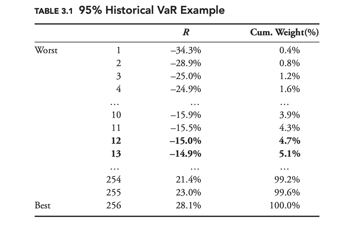
Now suppose we have 256 days of data, sorted from lowest to highest as in Table 3.1. We still want to calculate the 95% VaR, but 5% of 256 is 12.8. Should we choose the 12th day? The 13th? The more conservative approach is to take the 12th point, −15.0%. Another alternative is to interpolate between the 12th and 13th points, to come up with –14.92%. Unless there is a strong justification for choosing the interpolation method, the conservative approach is recommended.
No Maturity Vs Finite Lifespans
For securities with no maturity date such as stocks, the historical approach is incredibly simple. For derivatives, such as equity options, or other instruments with finite lifespans, such as bonds, it is slightly more complicated.
For a derivative, we do not want to know what the actual return series was, we want to know what the return series would have been had we held exactly the same derivative in the past.
For example, suppose we own an at-the-money put with two days until expiration. Two-hundred-fifty days ago, the option would have had 252 days until expiration, and it may have been far in or out of the money. We do not want to know what the return would have been for this option with 252 days to expiration. We want to know what the return would have been for an at-the-money put with two days to expiration, given conditions in the financial markets 250 days ago.
What we need to do is to generate a constant maturity or backcast series. These constant maturity series, or backcast series, are quite common in finance.
The easiest way to calculate the backcast series for an option would be to use a delta approximation. If we currently hold a put with a delta of −30%, and the underlying return 250 days ago was 5%, then our backcast return for that day would be −1.5% = −30% × 5%.
A more accurate approach would be to fully reprice the option, taking into account not just changes in the underlying price, but also changes in implied volatility, the risk-free rate, the dividend yield, and time to expiration. Just as we could approximate option returns using delta, we could approximate bond returns using DV01, but a more accurate approach would be to fully reprice the bond based on changes in the relevant interest rates and credit spreads.
Parametric Vs Historical Approach
The delta-normal approach is an example of what we call a parametric model. This is because it is based on a mathematically defined, or parametric, distribution (in this case, the normal distribution). By contrast, the historical approach is non-parametric. We have not made any assumptions about the distribution of historical returns.
There are advantages and disadvantages to both approaches. The historical approach easily reproduces all the quirks that we see in historical data: changing standard deviation, skewness, kurtosis, jumps, etc. Developing a parametric model that reproduces all of the observed features of financial markets can be very difficult. At the same time, models based on distributions often make it easier to draw general conclusions. In the case of the historical approach, it is difficult to say if the data used for the model are unusual because the model does not define usual.
Hybrid VaR (Historical & Decay Factor)
The historical model is easy to calculate and reproduces all the quirks that we see in historical data, but it places equal weight on all data points. If risk has increased recently, then the historical model will likely underestimate current risk. The delta-normal model can place more weight on more recent data by calculating standard deviation using a decay factor. The calculation with a decay factor is somewhat more difficult, but not much. Even with the decay factor, the delta-normal model still tends to be inaccurate because of the delta and normal assumptions.
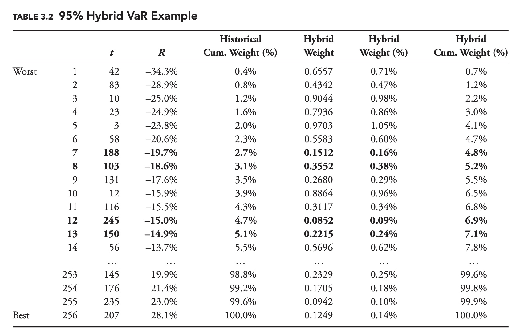
Can we combine the advantages of the historical model with the advantages of a decay factor? The hybrid approach to VaR does exactly this. Just as we did with standard deviation in Chapter 2, we can place more weight on more recent points when calculating VaR by using a decay factor. If we were calculating standard historical VaR at the 95% confidence level, then 5% of the data points would be on one side of our VaR estimate, and 95% would be on the other side.
With hybrid VaR it is not the number of points that matters, but their weight. With hybrid VaR, 5% of the total weight of the data points is on one side, and 95% is on the other.
Mechanically, in order to calculate hybrid VaR, we start by assigning a weight to each data point. If our decay factor was 0.98, then we would assign a weight of 1 to the most recent date, 0.98 to the previous day, 0.982 to the day before that, and so on. Next, we divide these weights by the sum of all the weights, to get a percentage weight for each day. Then we sort the data based on returns. Finally, we determine our estimate of VaR, by adding up the percentage weights, starting with the worst return, until we get to the desired confidence level. If our confidence level was 95%, then we would stop when the sum of the percentage weights was equal to 5%.
Monte Carlo Simulation
Monte Carlo simulations are widely used throughout finance, and they can be a very powerful tool for calculating VaR.
For simple scenarios, MCS is less efficient as parametric methods like delta-normal method. The real power of Monte Carlo simulations is in more complex settings, where instruments are nonlinear, prices are path dependent, and distributions do not have well-defined inverses. Also, as we will see in subsequent chapters when we extend our VaR framework to portfolios of securities, even very simple portfolios can have very complex distributions.
Monte Carlo simulations can also be used to calculate VaR over multiple periods. In the preceding example, if instead of being interested in the one-day VaR, we wanted to know the four-day VaR, we could simply generate four one-day log returns, using the same distribution as before, and add them together to get one four-day return. We could repeat this process 1,000 times, generating a total of 4,000 one-day returns. As with the one-day example, in this particular case, there are more efficient ways to calculate the VaR statistic. That said, it is easy to imagine how multi-day scenarios could quickly become very complex. What if your policy was to reduce your position by 50% every time you suffered a loss in excess of 3%? What if returns exhibited serial correlation?
Working with Multiple Periods:
Monte Carlo simulations are usually based on parametric distributions, but we could also use nonparametric methods, randomly sampling from historical returns. Continuing with our gold example, if we had 500 days of returns for gold, and we wanted to calculate the four-day VaR, we could randomly pick a number from 1 to 500, and select the corresponding historical return. We would do this four times, to create one four-day return. We can repeat this process, generating as many four-day returns as we desire. The basic idea is very simple, but there are some important details to keep in mind.
First, generating multi-period returns this way involves what we call sampling with replacement. Pretend that the first draw from our random number generator is a 10, and we select the 10th historical return. We don’t remove that return before the next draw. If, on the second draw, our random number generator produces 10 again, then we select the same return. If we end up pulling 10 four time in a row, then our four-day return will be composed of the same 10th return repeated four times.
Even though we only have 500 returns to start out with, there are $500^4$, or 62.5 billion, possible four-day returns that we can generate this way. This method of estimating parameters, using sampling with replacement, is often referred to as bootstrapping.
The second detail that we need to pay attention to is serial correlation and changes in the distribution over time. We can only generate multi-period returns in the way just described if single-period returns are independent of each other and volatility is constant over time.
Suppose that this was not the case, and that gold tends to go through long periods of high volatility followed by long periods of low volatility.
A simple solution to this problem: Instead of generating a random number from 1 to 500, generate a random number from 1 to 497, and then select four successive returns. If our random number generator generates 125, then we create our four-day return from returns 125, 126, 127, and 128.
While this method will more accurately reflect the historical behavior of volatility, and capture any serial correlation, it greatly reduces the number of possible returns from 62.5 billion to 497, which effectively reduces the Monte Carlo simulation to the historical simulation method.
Another possibility is to try to normalize the data to the current standard deviation. If we believe the current standard deviation of gold is 10% and that the standard deviation on a certain day in the past was 5%, then we would simply multiply that return by two. While this approach gets us back to the full 62.5 billion possible four-day returns for our 500-day sample, it requires us to make a number of assumptions in order to calculate the standard deviation and normalize the data.
Cornish-Fisher VaR
The delta-normal VaR model approximate the underlying returns with only the greek Delta. The Cornish-Fisher VaR model also incorporates gamma and theta.
To start with, we introduce some notation. Define the value of an option as V, and the value of the option’s underlying security as U. Next, define the option’s exposure-adjusted Black-Scholes-Merton Greeks as
\[\tilde{\Delta}=\frac{d V}{d U} U=\Delta U\] \[\tilde{\Gamma}=\frac{d^{2} V}{d U^{2}} U^{2}=\Gamma U^{2}\] \[\theta=\frac{d V}{d t}\]Given a return on the underlying security, R, we can approximate the change in value of the option using the exposure-adjusted Greeks as
\[d V \approx \tilde{\Delta} R+\frac{1}{2} \tilde{\Gamma} R^{2}+\theta d t\]If the returns of the underlying asset are normally distributed with a mean of zero and a standard deviation of $\sigma$, then we can calculate the moments of dV. The first three central moments and skewness of dV are
\[\begin{aligned} \mu_{d V} &=\mathrm{E}[d V]=\frac{1}{2} \tilde{\Gamma} \sigma^{2}+\theta d t \\ \sigma_{d V}^{2} &=\mathrm{E}\left[(d V-\mathrm{E}[d V])^{2}\right]=\tilde{\Delta}^{2} \sigma^{2}+\frac{1}{2} \tilde{\Gamma}^{2} \sigma^{4} \\ \mu_{3, d V} &=3 \tilde{\Delta}^{2} \tilde{\Gamma} \sigma^{4}+\tilde{\Gamma}^{3} \sigma^{6} \\ s_{d V} &=\frac{\mu_{3, d V}}{\sigma_{d V}^{3}} \end{aligned}\]$\mu_{3, d V}$ is the third central moment, and $s_{dV}$ is the skewness. Notice that even though the distribution of the underlying security’s returns is symmetrical, the distribution of the change in value of the option is skewed ($s_{dV} \neq 0$ ).
This makes sense, given the asymmetrical nature of an option payout function. That the Cornish-Fisher model captures the asymmetry of options is an advantage over the delta-normal model, which produces symmetrical distributions for options.
The central moments can be combined to approximate a confidence interval using a Cornish-Fisher expansion, which can in turn be used to calculate an approximation for VaR.
The Cornish-Fisher VaR (defined as return) of the an option is given by:
\[V a R=-\mu_{d V}-\sigma_{d V}\left[m+\frac{1}{6}\left(m^{2}-1\right) s_{d V}\right]\]where m corresponds to the distance in standard deviations for our VaR confidence level based on a normal distribution (e.g., m = −1.64 for 95% VaR).
As we would expect, increasing the standard deviation, $\sigma_{dV}$ , will tend to increase VaR (remember m is generally negative).
As we would also expect, the more negative the skew of the distribution the higher the VaR tends to be (in practice, $m^2 − 1$ will tend to be positive).
Unfortunately, beyond this, the formula is far from intuitive, and its derivation is beyond the scope of this book. As is often the case, the easiest way to understand the approximation, may be to use it. The following sample problem provides an example.
Sample Problem
Question: You are asked to evaluate the risk of a portfolio containing a single call option with a strike price of 110 and three months to expiration. The underlying price is 100, and the risk-free rate is 3%. The expected and implied standard deviations are both 20%. Calculate the one-day 95% VaR using both the delta-normal method and the Cornish-Fisher method. Use 365 days per year for theta and 256 days per year for standard deviation.
Answer:
To start with we need to calculate the Black-Scholes-Merton delta, gamma, and theta. These can be calculated in a spreadsheet or using other financial applications.
\[\begin{aligned} \Delta=& 0.2038\\ \Gamma=& 0.0283\\ \theta=& -6.2415 \end{aligned}\]The one-day standard deviation and theta can be found as follows:
\[\sigma_{d}=\frac{20 \%}{\sqrt{256}}=1.25 \%\] \[\theta_{d}=\left(\frac{-6.2415}{365}\right)=-0.0171\]Using m = −1.64 for the 5% confidence level of the normal distribution, the delta-normal approximation is
\[-V a R=m \sigma_{d} S \Delta+\theta_{d}=-1.64 \times 1.25 \% \times 100 \times 0.2038-0.0171=-0.4361\]For the Cornish-Fisher, approximation, we first calculate the exposure-adjusted Greeks:
\[\begin{aligned} \tilde{\Delta}&= \Delta U =20.3806\\ \tilde{\Gamma}&= \Gamma U^2 =283.1397 \end{aligned}\]Next, we calculate the mean, standard deviation, and skewness for the change in option value:
\[\begin{aligned} \mu_{d V} &=\frac{1}{2} \tilde{\Gamma} \sigma_{d}^{2}+\theta_{d}=\frac{1}{2} \times 283.1379 \times(1.25 \%)^{2}-0.0171=0.00503 \\ \sigma_{d V}^{2} &=\tilde{\Delta}^{2} \sigma_{d}^{2}+\frac{1}{2} \tilde{\Gamma}^{2} \sigma_{d}^{4}=20.3806^{2} 1.25 \%^{2}+\frac{1}{2} 283.1397^{2} 1.25 \%^{4}=0.06588 \\ \sigma_{d v} &=\sqrt{0.06588}=0.256672 \\ \mu_{3, d V} &=3 \tilde{\Delta}^{2} \tilde{\Gamma} \sigma_{d}^{4}+\tilde{\Gamma}^{3} \sigma_{d}^{6} \\ &=3 \times 20.3806^{2} \times 283.1379 \times 1.25 \%^{4}+283.1379^{3} \times 1.25 \%^{6} \\ &=0.0087 \\ s_{d V} &=\frac{\mu_{3, d V}}{\sigma_{d V}^{3}}=\frac{0.0087}{0.256672^{3}}=0.51453 \end{aligned}\]We then plug the moments into our Cornish-Fisher approximation:
\[\begin{aligned}-V_{a} R &=\mu_{d V}+\sigma_{d V}\left[m+\frac{1}{6}\left(m^{2}-1\right) s_{d V}\right] \\ &=0.00502+0.256672\left[-1.64+\frac{1}{6}\left(-1.64^{2}-1\right) 0.514528\right] \\ &=-0.3796 \end{aligned}\]The one-day 95% VaR for the Cornish-Fisher method is a loss of 0.3796, compared to a loss of 0.4316 for the delta-normal approximation. It turns out that in this particular case the exact answer can be found using the Black-Scholes-Merton equation. Given the assumptions of this sample problem, the actual one-day 95% VaR is 0.3759. In this sample problem, the Cornish-Fisher approximation is very close to the actual value, and provides a much better approximation than the delta-normal approach.
In certain instances, the Cornish-Fisher approximation can be extremely accurate. In practice, it is much more likely to be accurate if we do not go too far out into the tails of the distribution. If we try to calculate the 99.99% VaR using Cornish-Fisher, even for a simple portfolio, the result is unlikely to be as accurate as what we saw in the preceding sample problem. One reason is that our delta-gamma approximation will be more accurate for small returns. The other is that returns are much more likely to be well approximated by a normal distribution closer to the mean of a distribution. As we will see in the next section, there are other reasons why we might not want to calculate VaR too far out into the tails.
Backtesting
How it generally works?
An obvious concern when using VaR is choosing the appropriate confidence interval. As mentioned, 95% has become a very popular choice in risk management. In some settings there may be a natural choice, but, most of the time, the specific value chosen for the confidence level is arbitrary.
A common mistake for newcomers is to choose a confidence level that is too high. Naturally, a higher confidence level sounds more conservative. It is tempting to believe that the risk manager using the 99.9% confidence level is concerned with more serious, riskier outcomes, and is therefore doing a better job.
The problem is that, as we go further and further out into the tail of the distribution, we become less and less certain of the shape of the distribution.
In most cases, the assumed distribution of returns for our portfolio will be based on historical data. If we have 1,000 data points, then there are 50 data points to back up our 95% confidence level, but only one to back up our 99.9% confidence level. As with any parameter, the variance of our estimate of the parameter decreases with the sample size. One data point is hardly a good sample size on which to base a parameter estimate.
A related problem has to do with backtesting. Good risk managers should regularly backtest their models. Backtesting entails checking the predicted outcome of a model against actual data. Any model parameter can be backtested.
In the case of VaR, backtesting is easy. When assessing a VaR model, each period can be viewed as a Bernoulli trial. Either we observe an exceedance or we do not. In the case of one-day 95% VaR, there is a 5% chance of an exceedance event each day, and a 95% chance that there is no exceedance. In general, for a confidence level (1 − p), the probability of observing an exceedance is p. If exceedance events are independent, then over the course of n days the distribution of exceedances will follow a binomial distribution
\[P[K=k]=C_n^k p^k (1-p)^{n-k}\]We can reject the VaR model if the number exceedance is too high or too low.
Backtesting VaR models is extremely easy, but what would happen if we were trying to measure one-day VaR at the 99.9% confidence level. Four years is approximately 1,000 business days, so over four years we would expect to see just one exceedance. We could easily reject the model if we observed a large number of exceedances, but what if we did not observe any?
After four years, there would be a 37% probability of observing zero exceedances. Maybe our model is working fine, but maybe it is completely inaccurate and we will never see an exceedance. How long do we have to wait to reject a 99.9% VaR model if we have not seen any exceedances? Approximately 3,000 business days or 12 years.
At the 99.9% confidence level, the probability of not seeing a single exceedance after 3,000 business days is a bit less than 5%. It is still possible that the model is correct at this point, but it is unlikely.
Twelve years is too long to wait to know if a model is working or not. By contrast, for a 95% VaR model we could reject the model with the same level of confidence if we did not observe an exceedance after just three months. If our confidence level is too high, we will not be able to backtest our VaR model and we will not know if it is accurate.
The probability of a VaR exceedance should also be conditionally independent of all available information at the time the forecast is made. In other words, if we are calculating the 95% VaR for a portfolio, then the probability of an exceedance should always be 5%. The probability shouldn’t be different because today is Tuesday, because yesterday it was sunny, or because your firm has been having a good month. Importantly, the probability should not vary because there was an exceedance the previous day or because risk levels are elevated.
Serial Correlation
A common problem with VaR models in practice is that exceedances often end up being serially correlated. When exceedances are serially correlated, you are more likely to see another exceedance in the period immediately after an exceedance. {: .align-center}
To test for serial correlation in exceedances, we can look at the periods immediately {: .align-center}following any exceedance events. The number of exceedances in these periods should also follow a binomial distribution. For example, pretend we are calculating the one-day 95% VaR for a portfolio, and we observed 40 exceedances over the past 800 days. To test for serial correlation in the exceedances, we look at the 40 days immediately following the exceedance {: .align-center}events and count how many of those were also exceedances.
In other words, we count the number of back-to-back exceedances. Because we are calculating VaR at the 95% confidence level, of the 40 day-after days, we would expect that 2 of them (5% × 40 = 2) would also be exceedances. The actual number of these day-after exceedances should follow a binomial distribution with n = 40 and p = 5%.
Independent with the current risk level
Another common problem with VaR models in practice is that exceedances tend to be correlated with the level of risk. It may seem counterintuitive, but we should be no more or less likely to see VaR exceedances in years when market volatility is high compared to when it is low.
Positive correlation between exceedances and risk levels can happen when a model does not react quickly enough to changes in risk levels. Negative correlation can happen when model windows are too short, and the model over reacts.
To test for correlation between exceedances and the level of risk, we can divide our exceedances into two or more buckets, based on the level of risk. As an example, pretend we have been calculating the one-day 95% VaR for a portfolio over the past 800 days. We could divide the sample period in two, placing the 400 days with the highest forecasted VaR in one bucket and the 400 days with the lowest forecasted VaR in the other. We would expect each 400-day bucket to contain 20 exceedances: 5% × 400 = 20. The actual number of exceedances in each bucket should follow a binomial distribution with n = 400, and p = 5%.
Coherent Risk Measures
At this point we have introduced two widely used measures of risk, standard deviation and value at risk (VaR). Before we introduce any more, it might be worthwhile to ask what qualities a good risk measure should have.
In 1999 Philippe Artzner and his colleagues proposed a set of axioms that they felt any logical risk measure should follow. They termed a risk measure that obeyed all of these axioms coherent. As we will see, while VaR has a number of attractive qualities, it is not a coherent risk measure.
A coherent risk measure is a function $\varrho$ that satisfies properties of monotonicity, sub-additivity, homogeneity, and translational invariance.
Properties of Coherent Risk Measures
Consider a random outcome ${\displaystyle X}$ viewed as an element of a linear space $\mathcal{L}$ of measurable functions, defined on an appropriate probability space. A functional \(\varrho : \mathcal{L} → {\displaystyle \mathbb {R} \cup \{ +\infty \}}\) is said to be coherent risk measure for $ \mathcal{L}$ if it satisfies the following properties:
Normalized
\[\varrho(0) = 0\]That is, the risk of holding no assets is zero.
Monotonicity
\[\mathrm{If}\; Z_1,Z_2 \in \mathcal{L} \;\mathrm{and}\; Z_1 \leq Z_2 \; \mathrm{a.s.} ,\; \mathrm{then} \; \varrho(Z_1) \geq \varrho(Z_2)\]Sub-additivity
\[\mathrm{If}\; Z_1,Z_2 \in \mathcal{L} ,\; \mathrm{then}\; \varrho(Z_1 + Z_2) \leq \varrho(Z_1) + \varrho(Z_2)\]Indeed, the risk of two portfolios together cannot get any worse than adding the two risks separately: this is the diversification principle. In financial risk management, sub-additivity implies diversification is beneficial. The sub-additivity principle is sometimes also seen as problematic.
Positive homogeneity
\[\mathrm{If}\; \alpha \ge 0 \; \mathrm{and} \; Z \in \mathcal{L} ,\; \mathrm{then} \; \varrho(\alpha Z) = \alpha \varrho(Z)\]Loosely speaking, if you double your portfolio then you double your risk. In financial risk management, positive homogeneity implies the risk of a position is proportional to its size.
Translation invariance
If A is a deterministic portfolio with guaranteed return a and $Z \in \mathcal{L}$ then
\[\varrho(Z + A) = \varrho(Z) - a\]Market Risk: Extreme Value Theory
For example, if you had 2,000 historical daily returns, then there would be 100 20-day periods, each with a worst day. You could then use this worst-day series to make a prediction for what the worst day will be over the next 20 days.
You could even use the distribution of worst days to construct a confidence interval. For example, if the 10th worst day in our 100 worst-day series is −5.80%, you could say that there is a 10% chance that the worst day over the next 20 days will be less than or equal to −5.80%. This is the basic idea behind extreme value theory (EVT), that extreme values (minimums and maximums) have distributions that can be used to make predictions about future events.
Approaches to sampling historical Data for EVT
There are two basic approaches to sampling historical data for EVT.
The approach outlined above, where we divide the historical data into periods of equal length and determine the worst return in each period, is known as the block-maxima approach.
Another approach, known as the peaks-over-threshold (POT) approach, is similar, but only makes use of returns that exceed a certain threshold. The POT approach has some nice technical features, which has made it more popular in recent years, but the block-maxima approach is easier to understand. For this reason, we will focus primarily on the block-maxima approach.
Figure 4.2 shows the distribution of minimum daily returns generated in two Monte Carlo simulations. In each case, 40,000 returns were generated and divided into 20-day periods, producing 2,000 minimum returns. In the first simulation, the daily returns were generated by a normal distribution with a mean of 0.00% and a standard deviation of 1.00%. In the second simulation, daily returns were generated using a fat-tailed Student’s t-distribution, with the same mean and standard deviation. The median of both distributions is very similar, close to {: .align-center}−1.80%, but, as we might expect, the fat-tailed t-distribution generates more extreme minimums. For example, the normal distribution generated only one minimum less than −4.00%, while the t-distribution generated 82.
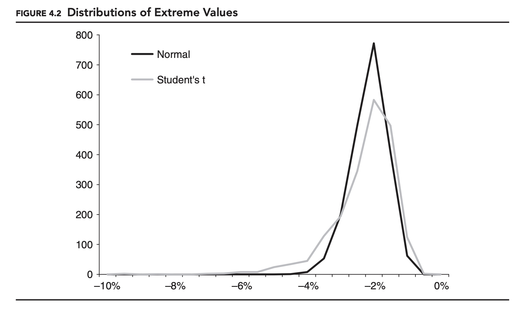
While the two distributions in Figure 4.2 are not exactly the same, they are similar in some ways. One of the most powerful results of EVT has to do with the shape of the distribution of extreme values for a random variable.
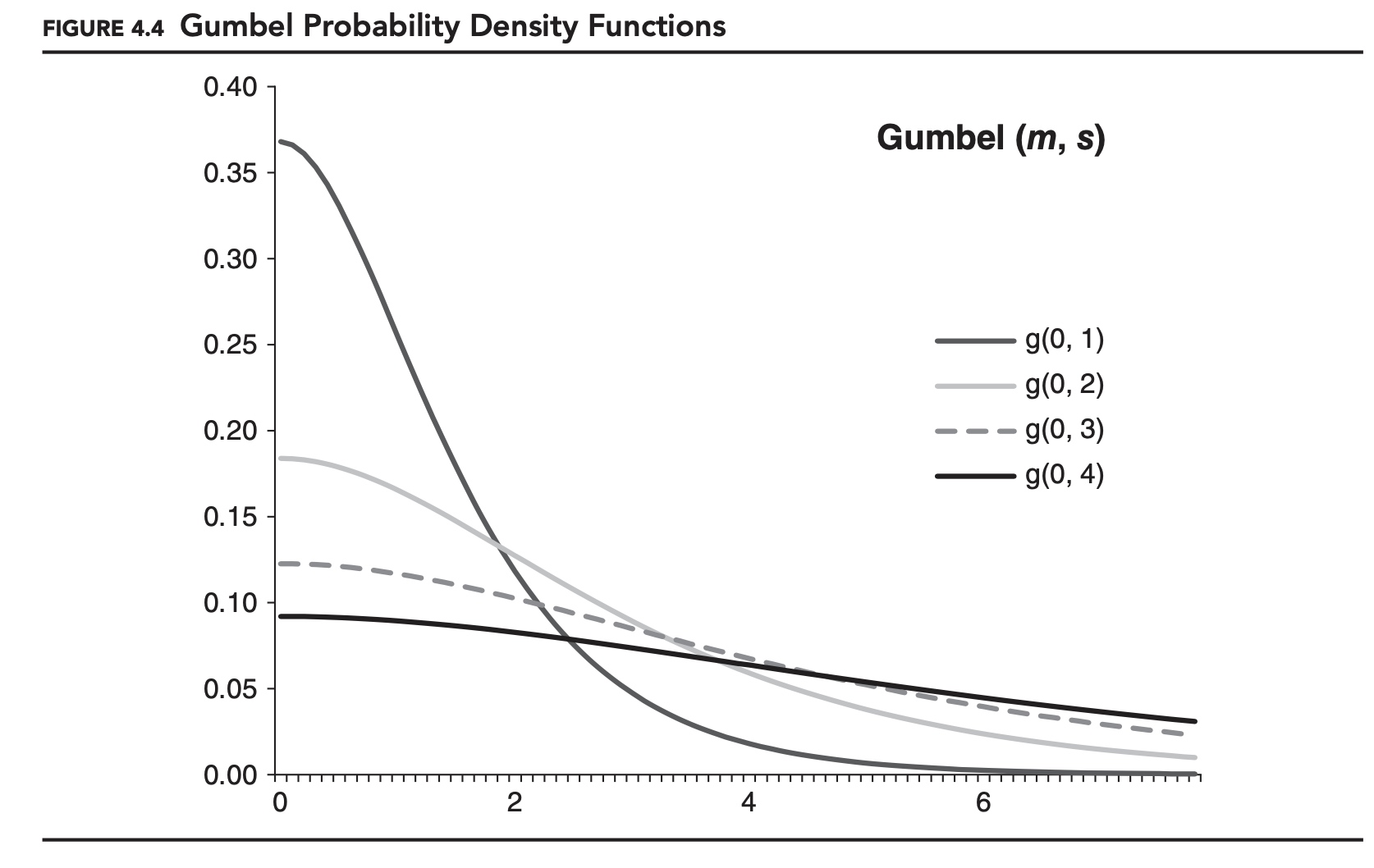
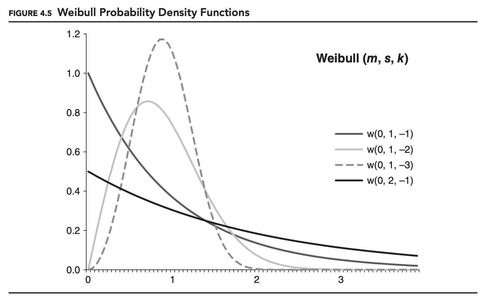
Provided certain conditions are met, the distribution of extreme values will always follow one of three continuous distributions, either the Fréchet, Gumbel, or Weibull distribution. These three distributions can be considered special cases of a more general distribution, the generalized extreme value distribution.
That the distribution of extreme values will follow one of these three distributions is true for most parametric distributions. One note of caution: This result will not be true if the distribution of returns is changing over time. The distribution of returns for many financial variables is far from constant, making this an important consideration when using EVT.
Table 4.1 shows the formulas for the probability density function (PDF) and cumulative distribution function (CDF) for each of the three EVT distributions, as well as for the generalized Pareto distribution, which we will come to shortly. Here, s is a scale parameter, k is generally referred to as a shape parameter, and m is a location parameter. The location parameter, m, is often assumed to be zero.
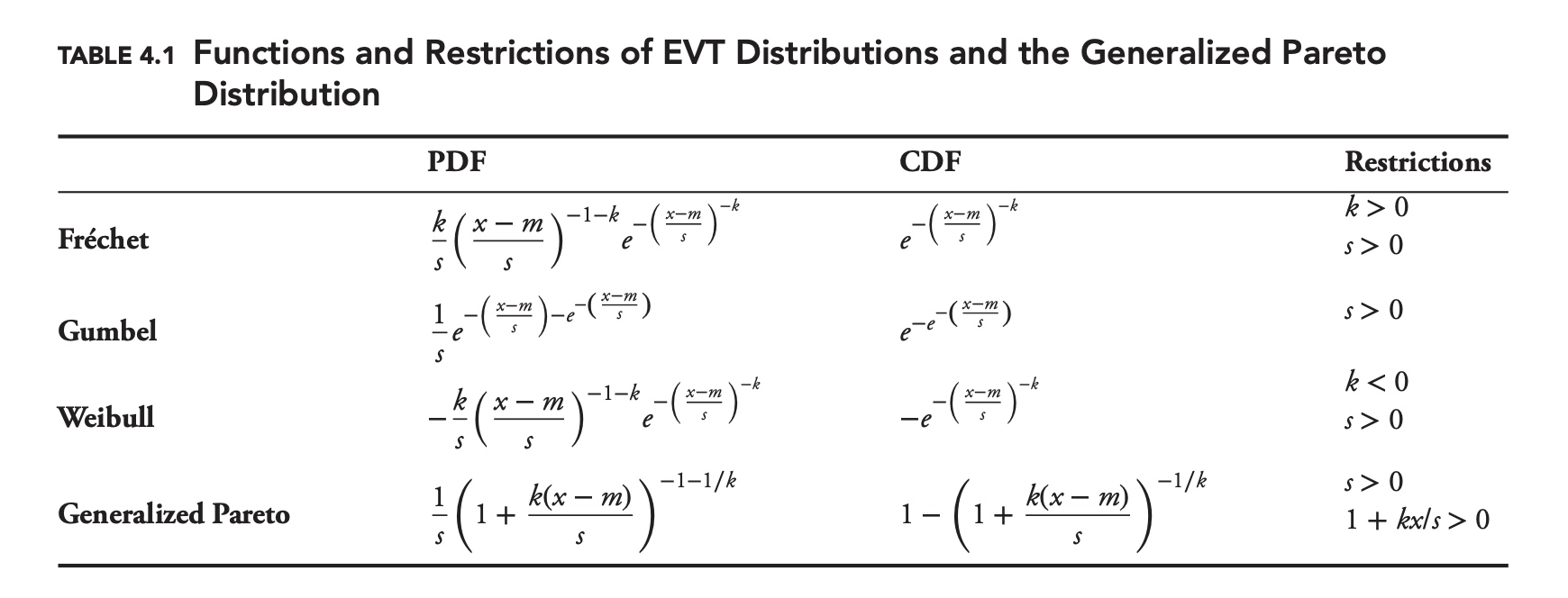
Figures 4.3, 4.4, and 4.5 show examples of the probability density function for each distribution. As specified here these are distributions for maximums, and m is the minimum for the distributions. If we want to model the distribution of minimums, we can either alter the formulas for the distributions, or simply reverse the signs of all of our data. The later approach is consistent with how we defined VaR and expected shortfall, working with losses instead of returns. This is the approach we will adopt for the remainder of this chapter.
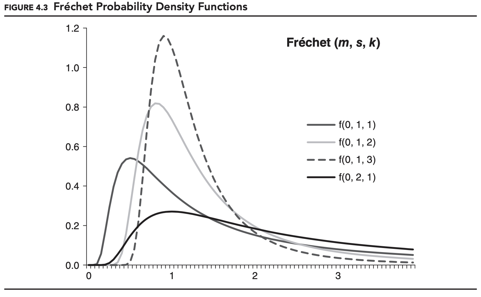

If the underlying data-generating process is fat-tailed, then the distribution of the maximums will follow a Fréchet distribution. This makes the Fréchet distribution a popular choice in many financial risk management applications.
Determination of the parameters
How do we determine which distribution to use and the values of the parameters? For block-maxima data, the most straightforward method is maximum likelihood estimation.
As an example, in Figure 4.6, 40,000 returns were generated using a Student’s t-distribution with a mean of 0.00% and a standard deviation of 1.00%. These were divided into 2,000 non-overlapping 20-day periods, just as in the previous example. The actual distribution in the figure shows the distribution of the 2,000 minimum points, with their signs reversed. (The distribution looks less smooth than in the previous figure because finer buckets were used.) On top of the actual distribution, we show the best-fitting Fréchet and Weibull distributions. As expected, the Fréchet distribution provides the best fit overall.
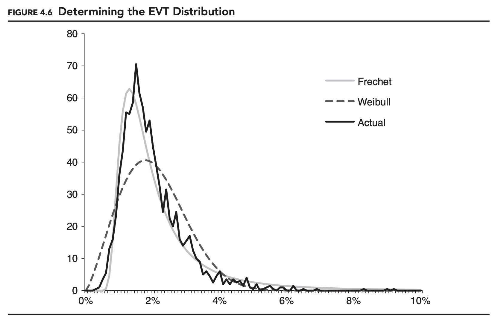
One problem with the block-maxima approach, as specified, is that all of the EVT distributions have a defined minimum. In Figure 4.6, both EVT distributions have a minimum of 0.00%, implying that there is no possibility of a maximum below 0.00% (or, reversing the sign, a minimum above 0.00%). This is a problem because in theory, the minimum in any month could be positive. In practice, the probability is very low, but it can happen.
The POT approach avoids this problem at the outset by considering only the distribution of extremes beyond a certain threshold. This and some other technical features make the POT approach appealing. One drawback of the POT approach is that the parameters of the EVT distribution are usually determined using a relatively complex approach that relies on the fact that, under certain conditions, the EVT distributions will converge to a Generalized Pareto distribution.
Sample Problem
Question: Based on the 2,000 maxima generated from the t-distribution, as described earlier, you have decided to model the maximum loss over the next 20 days using a Fréchet distribution with m = 0.000, s = 0.015, and k = 2.368. What is the probability that the maximum loss will be greater than 7.00%?
Answer: We can use the CDF of the Fréchet distribution from Table 4.1 to solve this problem.
\[P[L>0.07]=e^{-\left(\frac{x-m}{s}\right)^{-k}}=e^{-\left(\frac{0.07-0.00}{0.015}\right)^{-2.368}}=0.9743\]That is, given our distribution assumption, 97.43% of the distribution is less than 7.00%, meaning 2.57% of the distribution is greater or equal 7.00%. The probability that the maximum loss over the next 20 days will be greater than 7.00% is 2.57%.
Be careful how you interpret the EVT results. In the preceding example, there is a 2.57% chance that the maximum loss over the next 20 days will exceed 7%. It is tempting to believe that there is only a 2.57% chance that a loss in excess of 7% will occur tomorrow.
This is not the case. EVT is giving us a conditional probability, $P[L > 7\% \mid max]$, meaning the probability that the loss is greater than 7%, given that tomorrow is a maximum. This is not the same as the unconditional probability, P[L > 7%]. These two concepts are related, though. Mathematically,
\[\mathrm{P}[L>7 \%]=\mathrm{P}[L>7 \% \mid \max ] \mathrm{P}[\max ]+\mathrm{P}[L>7 \% \mid \max ] \mathrm{P}[\overline{\mathrm{max}}]\]where we have used max to denote L not being the maximum. In our current example we are using a 20-day window, so the probability that any given day is a maximum is simply 1/20. Using this and the EVT probability, we have
\[\mathrm{P}[L>7 \%]=2.57 \% \frac{1}{20}+\mathrm{P}[L>7 \% \mid \max ] \frac{19}{20}\]The second conditional probability, $P[L > 7\% \mid max]$, must be less than or equal to the first conditional probability. This makes Equation 4.5 a weighted average of 2.57% and some- thing less than or equal to 2.57%, so we know the unconditional probability must be less than or equal to 2.57%,
\[\mathrm{P}[L>7 \%]\leq 2.57\%\]Combination of EVT and Parametric model
A popular approach at this point is to assume a parametric distribution for the non-extreme events. This combined approach can be viewed as describing a mixture distribution. For example, we might use a normal distribution to model the non-extreme values and a Fréchet distribution to model the extreme values.
Continuing with our example, suppose we use a normal distribution and determine that the probability that L is greater than 7%, when L is not the maximum, is 0.05%. The unconditional probability would then be 0.17%,
\[\mathrm{P}[L>7 \%]=2.57 \% \frac{1}{20}+0.05 \% \frac{19}{20}=0.13 \%+0.04 \%=0.17 \%\]If the parametric distribution does a good job at modeling the non-extreme values and the EVT distribution does a good job at modeling the extreme values, then we may be able to accurately forecast this unconditional probability using this combination approach. This combined approach also allows us to use EVT to forecast VaR and expected shortfall, something we cannot do with EVT alone.
There is a certain logic to EVT. If we are primarily concerned with extreme events, then it makes sense for us to focus on the shape of the distribution of extreme events, rather than trying to approximate the distribution for all returns. But, in the past some proponents of EVT have gone a step further and claimed that this focus allows them to be very certain about extremely rare events.
Once we have determined the parameters of our extreme value distribution, it is very easy to calculate the probability of losses at any confidence level. It is not uncommon to see EVT used as the basis of one-day 99.9% or even 99.99% VaR calculations, for example.
Recall the discussion on VaR back-testing, though. Unless you have a lot of data and are sure that the data generating process is stable, you are unlikely to be able to make these kinds of claims. This is a fundamental limit in statistics. There is no way to get around it.
The remarkable thing about EVT is that we can determine the distribution of the minimum or maximum even if we don’t know the distribution of the underlying data-generating process. But knowing the type of distribution is very different from knowing the distribution itself. It’s as if we knew that the distribution of returns for a security followed a lognormal distribution, but didn’t know the mean or standard deviation. If we know that extreme losses for a security follow a Fréchet distribution, but are highly uncertain about the parameters of the distribution, then we really don’t know much.
One requirement of EVT that is unlikely to be met in most financial settings is that the underlying data-generation process is constant over time. There are ways to work around this assumption, but this typically leads to more assumptions and more complication.
Though we did not mention it before, the EVT results are only strictly true in the limit, as the frequency of the extreme values approaches zero. In theory, the EVT distributions should describe the distribution of the maxima reasonably well as long as the frequency of the extreme values is sufficiently low. Unfortunately, defining “sufficiently low” is not easy, and EVT can perform poorly in practice for frequencies as low as 5%.
Market Risk: Beyond Correlation
Coskewness and Cokurtosis
Just as we generalized the concept of mean and variance to moments and central moments, we can generalize the concept of covariance to cross-central moments. The third and fourth standardized cross-central moments are referred to as coskewness and cokurtosis, respectively. Though used less frequently, higher-order cross moments can be very important in risk management.
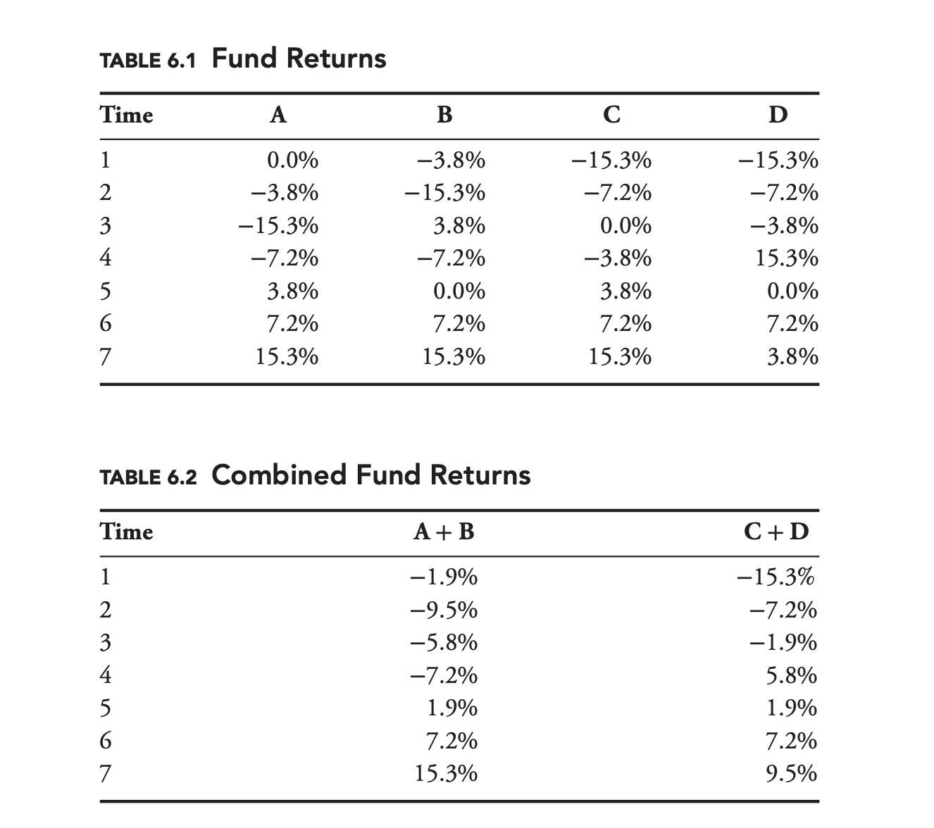
The two portfolios have the same mean and standard deviation, but the skews of the portfolios are different. Whereas the worst return for A + B is −9.5%, the worst return for C + D is −15.3%. As a risk manager, knowing that the worst outcome for portfolio C + D is more than 1.6 times as bad as the worst outcome for A + B could be very important.
It is very important to note that there is no way for us to differentiate between A + B and C + D, based solely on the standard deviation, variance, covariance, or correlation of the original four funds. That is, there is no way for us to differentiate between the two combined portfolios based solely on the information contained in a covariance matrix. As risk managers, we need to be on the lookout for these types of models, and to be aware of their limitations.
So how did two portfolios whose constituents seemed so similar end up being so differ- ent? One way to understand what is happening is to graph the two sets of returns for each portfolio against each other, as shown in Figures 6.1 and 6.2.
The two graphs share a certain symmetry, but are clearly different. In the first portfolio, A + B, the two managers’ best positive returns occur during the same time period, but their worst negative returns occur in different periods. This causes the distribution of points to be skewed toward the top-right of the chart. The situation is reversed for managers C and D:
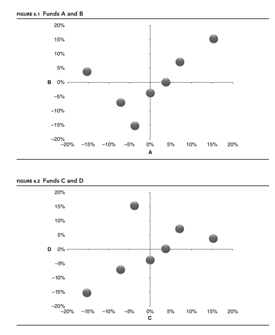
The reason the charts look different, and the reason the returns of the two portfolios are different, is because the coskewness between the managers in each of the portfolios is different. For two random variables, there are actually two nontrivial coskewness statistics.
For example, for managers A and B, we have
\[\begin{aligned} S_{A A B} &=\frac{\mathrm{E}\left[\left(A-\mu_{A}\right)^{2}\left(B-\mu_{B}\right)\right]}{\sigma_{A}^{2} \sigma_{B}} \\ S_{A B B} &=\frac{\mathrm{E}\left[\left(A-\mu_{A}\right)\left(B-\mu_{B}\right)^{2}\right]}{\sigma_{A} \sigma_{B}^{2}} \end{aligned}\]The complete set of sample coskewness statistics for the sets of managers is shown in Table 6.3.
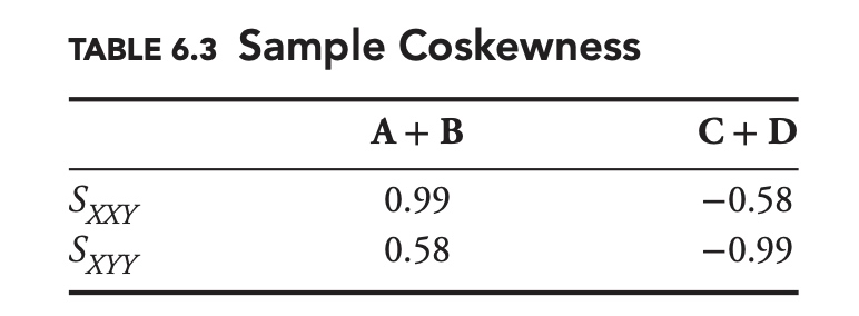
Both coskewness values for A and B are positive, whereas they are both negative for C and D. Just as with skewness, negative values of coskewness tend to be associated with greater risk.
Just as we defined coskewness, we can define cokurtosis. For two random variables, X and Y, there are three nontrivial cokurtosis statistics,
\[\begin{aligned} K_{X X X Y} &=\frac{\mathrm{E}\left[\left(X-\mu_{X}\right)^{3}\left(Y-\mu_{Y}\right)\right]}{\sigma_{X}^{3} \sigma_{Y}} \\ K_{X X Y Y} &=\frac{\mathrm{E}\left[\left(X-\mu_{X}\right)^{2}\left(Y-\mu_{Y}\right)^{2}\right]}{\sigma_{X}^{2} \sigma_{Y}^{2}} \\ K_{X Y Y Y} &=\frac{\mathrm{E}\left[\left(X-\mu_{X}\right)\left(Y-\mu_{Y}\right)^{3}\right]}{\sigma_{X} \sigma_{Y}^{3}} \end{aligned}\]Despite their obvious relevance to risk management, many standard risk models do not explicitly define coskewness or cokurtosis. One reason that many models avoid these higher-order cross moments is practical. As the number of variables increases, the number of nontrivial cross moments increases rapidly. With 10 variables there are 30 coskewness parameters and 65 cokurtosis parameters.
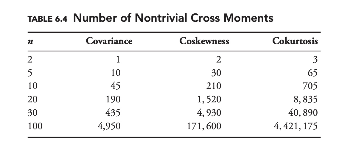
Table 6.4 compares the number of nontrivial cross moments for a variety of sample sizes. In most cases there is simply not enough data to calculate all of these higher-order cross moments.
Independent and Identically Distributed Random Variables
For a set of i.i.d. draws from a random variable, $x1, x_2, \cdots , x_n$, we define the sum, S, and mean, 𝜇, as
\[\begin{aligned} S&=\sum_{i=1}^n x_i\\ \mu &= \frac{S}{n} \end{aligned}\]Denoting the variance, standard deviation, third central moment, fourth central moment, skewness and kurtosis of a random variable x by $f (x)$, we define two constants, a and b, such that
\[\begin{aligned} f(S)&=af(x)\\ f(\mu) &= bf(x) \end{aligned}\]Table 6.10 provides values for a and b for each statistic. The second row contains the familiar square-root rule for standard deviation.
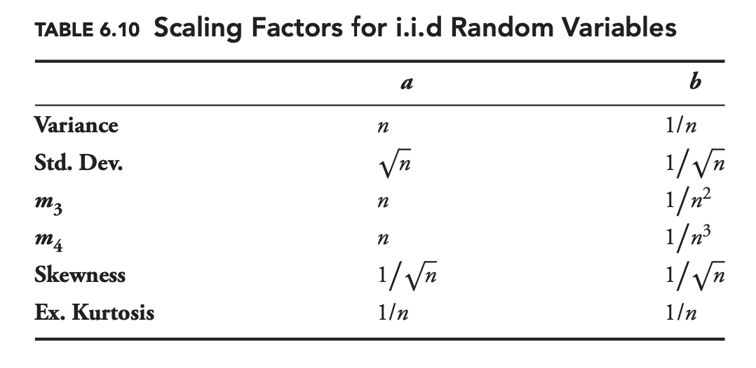
The last row tells us that the kurtosis of both the sum and mean of n i.i.d. variables is 1/n times the kurtosis of the individual i.i.d. variables. Interestingly, while the standard deviation and variance of the sum of n i.i.d. variable is greater than the standard deviation or variance of the individual random variables, respectively, the skewness and kurtosis are smaller. It is easy to understand why this is the case by noting that the value of a is n for all central moments.
By being familiar with the formulas in Table 6.10 you can often get a sense of whether or not financial variables are independent of each other. For example, consider the Russell 2000 stock index, which is a weighted average of 2,000 small-cap U.S. stocks. Even if the return distribution for each stock in the index was highly skewed, we would expect the distribution of the index to have very little skew if the stocks were independent (by table 6.10, the skewness of the index should be roughly $1/ \sqrt{2,000}≈1/45$ the mean skewness of the individual stocks).
In fact, the daily returns of the Russell 2000 exhibit significant negative skewness, as do the returns of most major stock indexes. This is possible because most stocks are influenced by a host of shared risk factors, and far from being independent of each other. In particular, stocks are significantly more likely to have large negative returns together, than they are to have large positive returns at the same time.
Market Risk: Risk Attribution
Factor Analysis
In risk management, factor analysis is a form of risk attribution, which attempts to identify and measure common sources of risk within large and complex portfolios. In a large, complex portfolio, it is sometimes far from obvious how much exposure a portfolio has to a given factor.
The classic approach to factor analysis can best be described as risk taxonomy. For each type of factor, each security is associated with one and only one factor. If we were trying to measure country exposures, each security would be assigned to a specific country—France, South Korea, the United States, and so on.
A limitation of the classic approach is that it is binary. A security is an investment in either China or Germany. This creates a problem in the real world. What do you do with a company that is headquartered in France, has all of its manufacturing capacity in China, sells its products in North America, and has listed shares on the London Stock Exchange? Is a company that sells consumer electronics a technology company or a retailer?
These kinds of obvious questions led to the development of various statistical approaches to factor analysis. One very popular approach is to associate each factor with an index, and then to use that index in a regression analysis to measure a portfolio’s exposure to that factor.
Another nice thing about factor analysis is that the factor exposures can be added across portfolios.
\[R_{\mathrm{A}}=\alpha_{A}+\beta_{A} R_{\mathrm{index}}+\varepsilon_{A}\] \[R_{\mathrm{B}}=\alpha_{B}+\beta_{B} R_{\mathrm{index}}+\varepsilon_{B}\] \[R_{\mathrm{A}+\mathrm{B}}=\left(\alpha_{A}+\alpha_{B}\right)+\left(\beta_{A}+\beta_{B}\right) R_{\mathrm{index}}+\left(\varepsilon_{A}+\varepsilon_{B}\right)\]Table 7.2 shows a sample exposure breakdown for an unspecified factor. Notice how the factor exposures are not necessarily proportional to the market values or even of the same sign
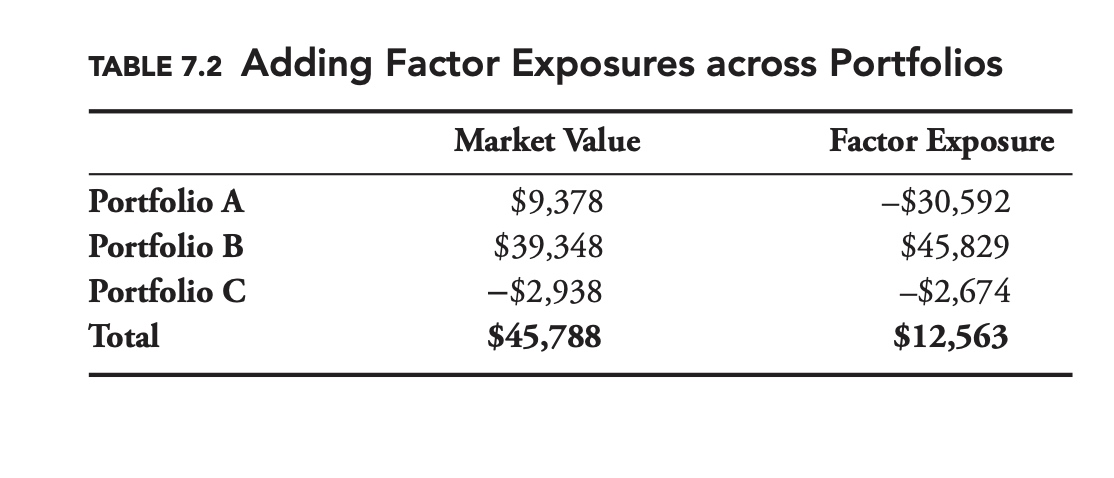
In addition to giving us the factor exposure, the factor analysis allows us to divide the risk of a portfolio into systematic and idiosyncratic components.
In this case, systematic risk refers to the risk in a portfolio that can be attributed to a factor. The risk that is not systematic (i.e., the risk that cannot be attributed to a factor) is referred to as idiosyncratic risk.
From our OLS assumptions, we know that $R_{index}$ and $\varepsilon$ are not correlated. Calculating the variance of $R_{portfolio}$ , we arrive at
\[\sigma^2_{portfolio}=\beta^2 \sigma^2_{index} +\sigma^2_{\varepsilon}\]Avoid multicollinearity
In theory, there is no reason why we cannot extend our factor analysis using multivariate regression analysis. In practice, many of the factors we are interested in will be highly correlated (e.g., most equity indexes are highly correlated with each other).
For example, if we are using a broad market index as a primary factor, then the spread between that index and a country factor might be an interesting secondary factor.
As outlined in the section on multicollinearity in Chapter 5, we can use the residuals from the regression of our secondary index on the primary index to construct a return series that is uncorrelated with the primary series.
Risks not Captured by public indexes
In theory, factors can be based on almost any kind of return series. The advantage of indexes based on publicly traded securities is that it makes hedging very straightforward. At the same time, there might be some risks that are not captured by any publicly traded index.
Some risk managers have attempted to resolve this problem by using statistical techniques, such as principal component analysis (PCA) or cluster analysis, to develop more robust factors. Besides the fact that these factors might be difficult to hedge, they might also be unstable, and it might be difficult to associate these factors with any identifiable macroeconomic variable.
Even using these statistical techniques, there is always the possibility that we have failed to identify a factor that is an important source of risk for our portfolio. Factor analysis is a very powerful tool, but it is not without its shortcomings.
Incremental VaR
A number of statistics have been developed to quantify the impact of a position or sub-portfolio on the total value at risk (VaR) of a portfolio. One such statistic is incremental VaR (iVaR). For a position with exposure wi, we define the iVaR of the position as
\[iVaR_i=\frac{d(VaR)}{dw_i} w_i \tag{7.4}\label{7.4}\]Here VaR is the total VaR of the portfolio. It is easier to get an intuition for iVaR if we rearrange Equation 7.4 as
\[d(VaR)=\frac{dw_i}{w_i} iVaR_i\tag{7.5}\label{7.5}\]If we have 200 of a security, and we add 2 to the position, then dwi/wi is 2/200 = 1%. On the left-hand side of the equation, d(VaR) is just the change in the VaR of the portfolio. Equation 7.5 is really only valid for infinitely small changes in wi, but for small changes it can be used as an approximation.
That iVaR is additive is true no matter how we calculate VaR, but it is easiest to prove for the parametric case, where we define our portfolio’s VaR as a multiple, m, of the portfolio’s standard deviation, $\sigma_P$.
Diversification
diversification score
One way to measure diversification is to compare the standard deviation of the securities in a portfolio to the standard deviation of the portfolio itself.
The diversification score is far from being a perfect measure of diversification. One shortcoming is that it is sensitive to how you group a portfolio.
diversification index
Meucci (2009) proposed measuring diversification using principal component analysis. More specifically, a portfolio with n securities will have n principal components. Of all of the principal components, the first explains the greatest amount of the variance in the portfolio, the second the second most, and so on.
When the portfolio has no diversification, either because the portfolio has only one security, or all of the securities are perfectly correlated with the same underlying risk factor, then the first principal component will explain all of the variance in the portfolio and N = 1.
At the other extreme, when the portfolio is maximally diversified, all of the principal components will explain an equal amount of the variance, and N = n.
Intuitively, N represents the actual number of diversified securities. Put another way, rather than counting securities, we should be counting how many independent sources of risk we have using our diversification index.
Risk-Adjusted Performance
For a security with expected return, $R_i$, and standard deviation, $\sigma_i$, given the risk-free rate, $R_rf$, the Sharpe ratio is
\[S_i=\frac{R_i-R_{rf}}{\sigma_i}=\frac{\mu_i}{\sigma_i}\]Naturally, if we wish to maximize the Sharpe ratio of our portfolio, at the margin we should choose the security with the highest incremental Sharpe $\Delta S_P= S_{P+\delta i}-S_P$.
Intuition
Intuitively, if a security and a portfolio are perfectly correlated, then it will only make sense to add the security to the portfolio if the security has a higher Sharpe ratio than the existing portfolio.
If the security has a lower Sharpe ratio, it might still make sense to add it if it provides enough diversification, if $\rho$ is low enough.
If $S_i^{\star}$ is negative, then adding the security to your portfolio will actually decrease the overall Sharpe ratio.
Choosing Statistics
This was the last of six chapters on market risk. Among other topics, we have looked at standard deviation, VaR, expected shortfall, extreme value theory (EVT), correlation, coskewness, copulas, stress testing, incremental VaR and diversification.
As we said before, no single risk statistic is perfect. All have their strengths and weaknesses. Standard deviation is very easy to understand and to calculate, but does not take into account the shape of the distribution. Expected shortfall places more emphasis on extreme negative outcomes, but it requires us to make certain model assumptions and is difficult to backtest.
Not all of these concepts are mutually exclusive. For example, we might be able to use copulas and EVT to improve our VaR forecast.
While there is not always one right answer, there is often a wrong answer. As our discussion of coskewness and copulas makes clear, if a joint distribution is not elliptical and we assume that it is, then we may severely underestimate risk. All of our models and statistics make certain assumptions. It is important that both the risk manager and portfolio manager understand the assumptions that underlie our models.
Modern financial markets are complex and move very quickly. The decision makers at large financial firms need to consider many variables when making decisions, often under considerable time pressure. Risk—even though it is a very important variable—will likely be only one of many variables that go into this decision-making process.
Credit Risk
Default Risk and Pricing
For a one-year zero-coupon bond, with probability of default D, and a loss given default L, the initial price is
\[V_0= (1-D)\frac{N}{1+R}+ D(1-L)\frac{N}{1+R}=(1-DL)\frac{N}{1+R}\]For the YTM (denoted as Y):
\[V_0=\sum_{t=1}^T \frac{c}{(1+Y)^t}+\frac{N}{(1+Y)^T}\]We have
\[1+Y=\frac{1+R}{1-DL} \implies Y=\frac{R+DL}{1-DL} \tag{8.7}\label{8.7}\]Determine the Probability of default
How do we determine the probability of default for a given bond issuer?
PD implied by market price
We could try to back out the default rate, based on observed market prices using an equation similar to Equation $\eqref{8.7}$. But, as discussed, because investors are risk averse, this will only give us the risk-neutral implied default rate, not the actual default rate.
Historical rate
We could look at the historical default rate for a bond issuer, but for any particular bond issuer, defaults are likely to be rare. Many bond issuers have never defaulted. If we are going to forecast the probability of default for a given issuer, we cannot rely on the history of defaults for that issuer. We will need some other approach.
Traditional Ratings Approach
The traditional approach to forecasting defaults is for rating agencies to assess the creditworthiness of an issuer.
To the extent that more highly rated issuers have been less likely to default than lower-rated issuers, the traditional approach seems to have worked historically. Table 8.2 shows the average five-year default rate for corporate bonds rated by Moody’s from 1920 to 2011. As expected, AAA bonds have defaulted at a lower rate than AA bonds, which have defaulted at a lower rate than A bonds, and so on.
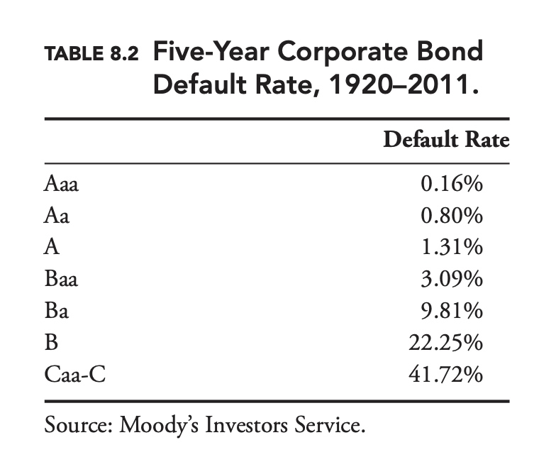
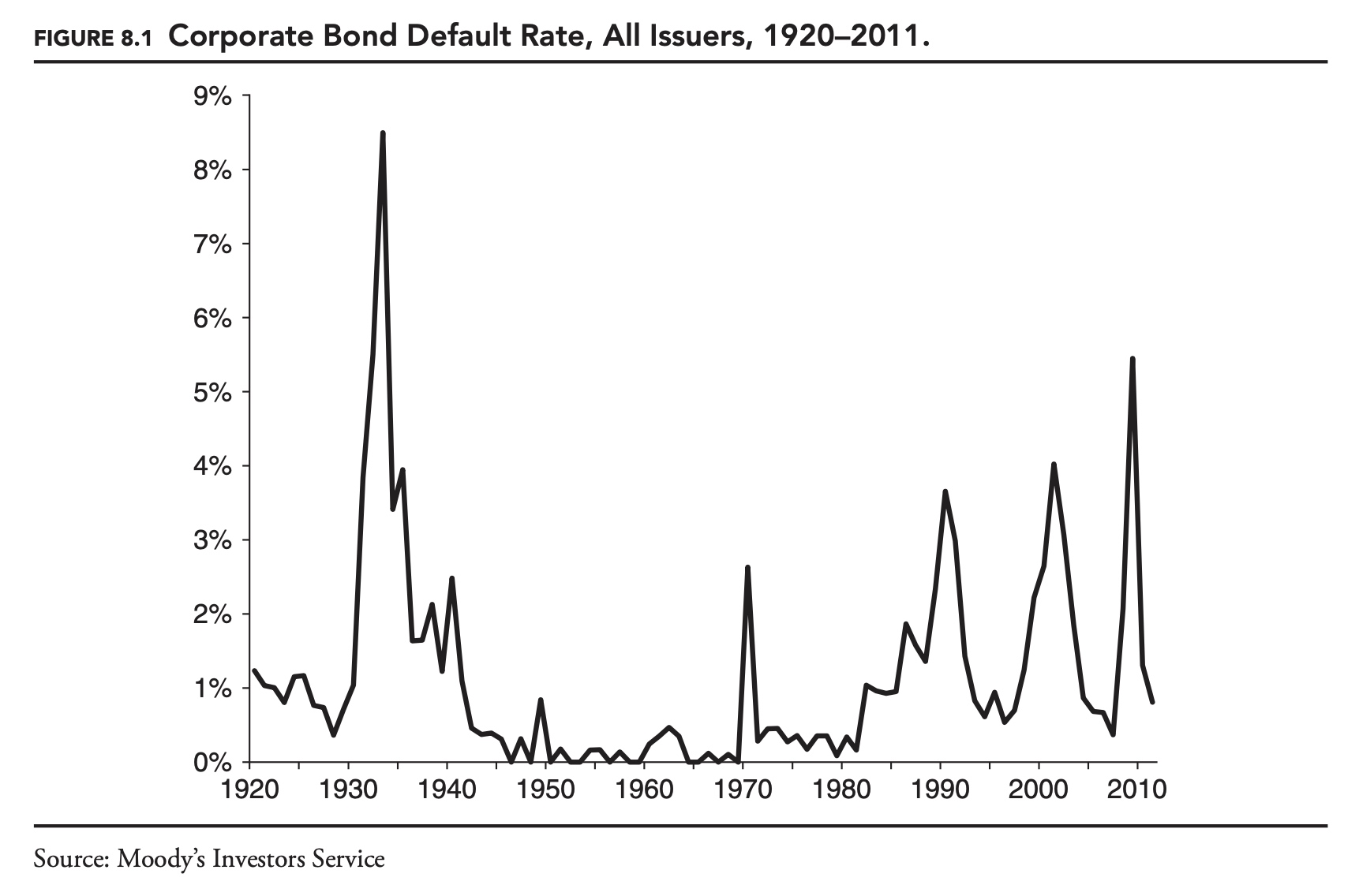
Over time default rates vary widely, overall and for individual letter ratings. Figure 8.1 shows the default rate for all corporate bonds between 1920 and 2011. The variation in default rates is driven largely by changes in the economic environment. As risk managers, if we were to base our forecast of default rates over the next year on long-run average default rates, our forecasts would be very inaccurate most of the time. Fortunately, some of the variation over time in default rates is predictable. The various rating agencies issue default forecasts on a regular basis. As with the ratings, these forecasts are based on both quantitative and qualitative inputs.
Transition Matrices
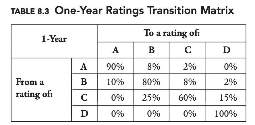
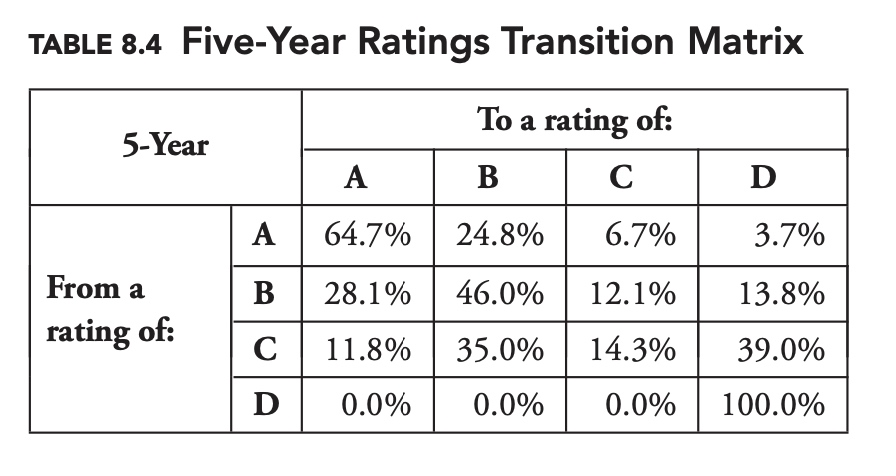
It turns out rather conveniently that we can calculate the complete two-year transition matrix by multiplying the one-year transition matrix by itself. If $T_1$ is our one-year transition matrix, and $T_n$ is our n-year transition matrix, then
\[T_n=T_1^n\]Quantitative Approach
Over time a number of practitioners and academics have tried to develop a more systematic, quantitative approach to predicting default. In this section we explore the widely used distance-to-default model, first proposed by Robert Merton in 1974.
As an equation, if we denote the enterprise value of the firm as $V_E$, and the value of the firm’s stock as S, and the value of its bonds by B, we have
\[V_E=S+B\]Merton’s great insight was to realize that we can view the equity holders as having a call option on the value of the firm. Viewed this way, the value of the equity, S, at the end of the year is
\[S=Max(V_E -B,0)\]In other words, the owning the stock of a firm is equivalent to owning a call option on the enterprise value of the firm, with a strike price equal to B, the value of the bonds.
Because we can observe the price of the equity in the stock market, and we know B, we can use the Black-Scholes-Merton option pricing formula to back out the market-implied volatility of the enterprise value. If we know the current enterprise value, and we know the expected volatility of the enterprise value, then we can easily determine the probability of default, which is the probability that the enterprise value will fall below B.
Rather than express the distance to default in dollar terms, what we really want to know is the probability of default. Assume the stock price follows a brownian motion, then in the risk-neutral world, by Ito-formula, we know:
\[\begin{aligned} \frac{dS_t}{s_t}&= rd_t + \sigma dw_t\\ \implies d (ln S_t)&=\frac{dS_t}{s_t} -\frac{1}{2} \frac{dS_t*dS_t}{S_t^2}\\ &=(r-\frac{1}{2}\sigma^2) dt + \sigma dw_t \end{aligned}\]If we now assume that the log returns of the enterprise value follow a normal distribution, then this is equivalent to asking how many standard deviations we are from default. Because we are using options pricing, we need to take into account the expected risk-neutral drift of the enterprise value, $(r-\sigma_V^2/2)T$, where r is the risk-free rate, $\sigma_V$ is the implied volatility of the enterprise value, and T is the time to expiration.
In order to default, the enterprise value must undergo a return of
\[ln(1 – S/VE_) =ln(B/V_E)=-ln(V_E/B)\]Finally, the standard deviation of the returns over the remaining life of the option is $\sigma_V \sqrt{T}$. Putting it together, the distance to default in standard deviations is
\[\Delta=\frac{-\ln \left(\frac{V_{E}}{B}\right)-\left(r-\frac{\sigma_{V}^{2}}{2}\right) T}{\sigma_{V} \sqrt{T}}=-d_{2}\]Here we have introduced the variable $−d_2$, which is the common designation for this quantity in the Black-Scholes-Merton model. Finally, to convert this distance to default into a probability of default, we simply use the standard normal cumulative distribution function, $P[D] = N(−d_2)$.
which method is better
Which approach is better? In practice, asset managers with large fixed-income holdings often use both ratings and quantitative models. They are also likely to supplement public ratings and commercially available quantitative models with their own internal ratings and models. One of the best examples of how the two approaches are viewed in practice can be seen in the history of KMV. Prior to 2002, KMV was one of the leading firms offering software and ratings based on Merton-type quantitative models. KMV suggested that its approach was superior to the approach of the rating agencies, and the rating agencies shot right back, insisting that their approach was in fact superior. In 2002, one of those rating agencies, Moody’s purchased KMV. Moody’s now offers products and services combining both approaches.
Liquidity Risk
In a crisis, liquidity can often make the difference between survival and disaster for a financial firm. We begin this chapter by defining liquidity risk before introducing measures and models that can help manage liquidity risk.
Simple Liquidity Measures
We begin by exploring some relatively simple liquidity measures. These measures fail to fully capture all aspects of liquidity risk, but they are easy to calculate and understand.
Weighted Average Days Volume
One of the simplest and most widely used measures of portfolio liquidity is the weighted average days’ volume, often referred to simply as the average days’ volume for a single security.
On the one hand, trading volumes often spike around news events, producing highly skewed distributions. Because of this, the median will tend to be more stable and more conservative. On the other hand, if these volume spikes are fairly common, or our trading horizon is sufficiently long, the mean may provide a better indication of how difficult it will be to liquidate a position. Because of this, and because average daily volume is such a commonly used expression, we will continue to use average to describe this particular statistic.
To get the weighted average days’ volume for a portfolio of securities, we can calculate a weighted average based on each position’s absolute market value.
The advantage of using weighted average days’ volume to summarize liquidity is that it is easy to calculate and easy to understand. That said, weighted average days’ volume is incredibly simplistic and leaves out many aspects of liquidity risk, which may be important.
Weighted average days’ volume works best when a portfolio is composed of similar securities with similar risk characteristics and similar trading volumes.
If a firm has a mix of highly liquid and highly illiquid securities, or if it has a mix of high-volatility and low-volatility securities, then we are likely to have to look beyond weighted average days’ volume in order to accurately gauge liquidity risk.
Liquidity Schedule
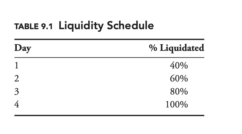
Table 9.1 provides an example. Here 40% of the portfolio can be liquidated within one day, and the entire portfolio can be liquidated within four days.
2 Steps to create a liquidity Table
- make an assumption about how quickly we can liquidate individual positions;
- calculate how much of each position we can liquidate each day.
- sum up the liquidation progress
As with weighted average days’ volume, there is no universally agreed-upon value. In practice a risk manager may look at more than one scenario, for example, a fast liquidation scenario and a slow liquidation scenario.
Liquidity Cost Models
Our standard market-risk model is based on market prices, which are often the midpoint of the bid-ask spread. When we go to sell a security, we will not receive this market price, but the ask price, which is slightly lower. This lower price will act to reduce our profit and loss (P&L). We can add this potential loss into the profit distribution due to market risk. We can then calculate the liquidity-adjusted value at risk (LVaR).
If we try to sell too much, we may push down the price and our profits further. In the first section we will ignore this potential source of loss and assume we can trade as much as we want at the current bid or ask price. In other words, we will assume that the price at which we can buy and sell securities is exogenous, and not impacted by our actions. In the second section, when we look at endogenous models, we will incorporate the potential impact of our own behavior on security prices.
Exogenous Liquidity Models
The difference between the market price and the price where we can buy or sell is equal to half the bid-ask spread. Given the bid-ask spread, the LVaR for a single unit of a security is just the standard VaR plus half the bid-ask spread. For n units of the security, we simply multiply the spread by n.
\[LVaR=VaR+n\frac{1}{2}(P_{aks}-P_{bid})\]Model the bid-ask spread
For extremely liquid securities, under normal market conditions, the bid-ask spread might be relatively stable. For less liquid securities, or in unsettled markets, the bid-ask spread may fluctuate significantly. Rather than using a fixed bid-ask spread, then, it may be appropriate to model the spread as a random variable. As with the distribution of market returns used to calculate our standard VaR, we can use either parametric or non-parametric distributions to model the bid-ask spread.
Correlation between spreads and market returns
When adding spread adjustments to our market risk distribution, it may be necessary to consider the correlation between spreads and market returns. In severe down markets, spreads will often widen. Depending on whether we are long or short, this correlation may make LVaR worse or better, compared to an assumption of no correlation. Spreads may also increase as market volatility increases.
Price spread vs percentage spread
If the bid and ask prices were 9.90 and 10.10, respectively, then the bid-ask spread would be 0.20. Quoting spreads in dollar terms like this is common practice in financial markets. When modeling spreads, though, it might be more appropriate to use percentage spreads.
In theory, we might expect percentage spreads to be more stable. In practice because securities trade in discrete increments, and because there are fixed costs associate with trading a unit of a security, the distribution of dollar spreads may in fact be more stable. This is another factor to consider when specifying a model.
Endogenous Liquidity Models
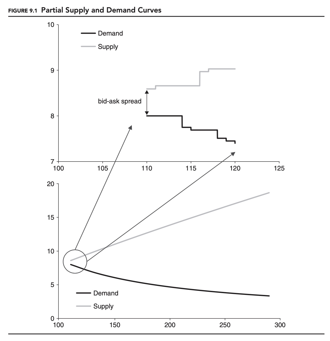
Financial securities, just like all other goods and services, are subject to the law of supply and demand. The higher the price of a security, the more sellers will be willing to sell, increasing the supply, but the less buyers will be willing to buy, decreasing the demand.
Figure 9.1 shows an example of a partial supply and demand curve for a security. Unlike the supply and demand curves that you might be familiar with from economics textbooks, these partial curves represent only the buyers and sellers who are unwilling to trade at the current price. These buyers and sellers represent potential liquidity in the market. The small gap between the two leftmost points on each curve represents the bid-ask spread. Because securities trade in discrete units (e.g., currently U.S. stocks trade in one-cent increments) when we look closely at these curves, they appear jagged. In the top half of Figure 9.1, we can see this clearly. If we zoom out, though, as in the bottom half of the figure, the curves start to look smooth. As we will see, even when markets are discrete, we often base our models on these smooth approximations.
A popular functional form for supply and demand curves is to choose constant elasticity. The elasticity, 𝜆, is the percentage change in quantity divided by the percentage change in price:
\[\lambda = \frac{dQ/Q}{dP/P}\]Once we know the elasticity of demand, it is a simple matter to calculate the impact of a given trade on the price of the security. This can then be translated into a loss, which can be added to the market VaR to arrive at the LVaR.
LVaR
LVaR is a compelling statistic for a number of reasons. It defines liquidity risk in terms of its impact on P&L, and it provides us with a single number which captures both market and liquidity risk.
It is not without its disadvantages, though. Spreads may be difficult to estimate for illiquid securities—the very securities that may pose the most liquidity risk—and estimating the supply or demand functions can be extremely difficult, even for liquid securities.
The uncertainty surrounding estimates of the liquidity adjustment could potentially swamp the overall estimate, turning a meaningful VaR statistic into a difficult-to-interpret LVaR statistic. In practice, LVaR is rarely a replacement for VaR; rather, it is reported in addition to VaR.
Even though the name is very similar to VaR, LVaR is fundamentally different. Whereas we can backtest VaR, comparing it to actual P&L on a regular basis, large liquidations are likely to happen infrequently. LVaR is likely to be very difficult to backtest.
Optimal Liquidation
When trying to liquidate a portfolio or part of a portfolio, there is always a trade-off between reducing risk and reducing liquidation costs.
With LVaR models, the standard approach is to choose an arbitrary liquidation horizon, which, in turn, determines the liquidation cost. The idea behind optimal liquidation is to let the model choose the time horizon, so that risk reduction and liquidation costs are balanced.
We start with a simple scenario. Imagine you are faced with a choice: You are long 100 of XYZ. Tomorrow there is a 50/50 chance that the price of XYZ will either increase or decrease by 10%. You can either sell the entire position today, or sell half today and half tomorrow. On either day, you can sell up to 55 at 2% below the market price. If you sell the 100 in one day you will need to sell at 4% below the market price. What should you do?
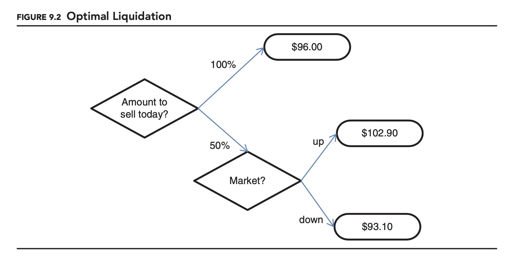
As summarized in Figure 9.2, if you sell everything today you are guaranteed to get 96. If you only sell 50% today you have a 50/50 chance of ending up with 102.90 or 93.10. This is an expected payout of 98. If you wait, you are better off on average, but you could be worse off. In this scenario, no choice is necessarily better than the other. Which is better depends on personal preference. More specifically, as we will see when we discuss behavioral finance, the choice depends on how risk averse you are. If you are extremely risk averse you will choose 96 with certainty. If you are less risk averse, you will choose to accept more risk for a slightly higher expected return. Determining the appropriate level of risk aversion to apply can make the optimal liquidation difficult to determine in practice.
Full-blown scenario analysis can be extremely complex. As with LVaR, we can use exogenous spreads or endogenous spreads, and consider the correlation of liquidity risk to other risk factors.
Comments