Chapter 7: Linear Regression Analysis
Univariate Linear Regression (One Regressor)
\[Y=\alpha +\beta X + \varepsilon\]As specified, X is known as the regressor or independent variable. Similarly, Y is known as the regressand or dependent variable. As dependent implies, traditionally we think of X as causing Y. This relationship is not necessary, and in practice, especially in finance, this cause-and-effect relationship is either ambiguous or entirely absent. In finance, it is often the case that both X and Y are being driven by a common underlying factor.
Note that, even it is called univariate linear regression, there are actually two features (1,X).
In our regression model, Y is divided into a systematic component, $\alpha + \beta X$, and an idiosyncratic component, $\varepsilon$.
Ordinary Least Square
The univariate regression model is conceptually simple. In order to uniquely determine the parameters in the model, though, we need to make some assumption about our variables.
By far the most popular linear regression model is ordinary least squares (OLS). OLS makes several assumptions about the form of the regression model, which can be summarized as follows:
A1: The relationship between the regressor and the regressand is linear.
A2: \(E[\varepsilon \vert X]=0\)
A3: \(Var[\varepsilon\vert X]=\sigma^2\)
A4: \(Cov[\varepsilon_i , \varepsilon_j ] = 0~ ∀i \neq j\)
A5: \(\varepsilon_i ∼ N(0,\sigma^2 )~\forall \varepsilon_i\)
A6: The regressor is nonstochastic.
A1: Linear
This assumption is not nearly as restrictive as it sounds.
1) Suppose we suspect that default rates are related to interest rates in the following way:
\[D=\alpha +\beta R^{3/4} + \varepsilon\]Because of the exponent on R, the relationship between D and R is clearly nonlinear. Still, the relationship between D and $R^{3/4}$ is linear.
2) As specified, the model implies that the linear relationship should be true for all values of D and R. In practice, we often only require that the relationship is linear within a given range.
A2: independence between ε and X
Assumption A2 implies that the error term is independent of X, i.e.:
\[Cov[X,\varepsilon]=0\]This because
\[E[\varepsilon X]=E[X* E_X [\varepsilon]]=E[X*0]=0\]A3: homoscedasticity
Assumption A3 states that the variance of the error term is constant. This property of constant variance is known as homoscedasticity, in contrast to heteroscedasticity, where the variance is nonconstant.
In finance, many models that appear to be linear often violate this assumption. As we will see in the next chapter, interest rate models often specify an error term that varies in relation to the level of interest rates.
A4: spherical errors
Assumption A4 states that the error terms for various data points should be uncorrelated with each other.
A random variable that has constant variance and is uncorrelated with itself is termed spherical. OLS assumes spherical errors.
A5: normally distributed
Assumption A5 states that the error terms in the model should be normally distributed. Many of the results of the OLS model are true, regardless of this assumption. This assumption is most useful when it comes to defining confidence levels for the model parameters.
A6: Nonstochastic
Finally, assumption A6 assumes that the regressor is nonstochastic, or nonrandom.
In reality, both the index’s return and the stock’s return are random variables, determined by a number of factors, some of which they might have in common. At some point, the discussion around assumption A6 tends to become deeply philosophical. From a practical standpoint, most of the results of OLS hold true, regardless of assumption A6. In many cases the conclusion needs to be modified only slightly.
An application of A2
\[\beta=\frac{\operatorname{Cov}[X, Y]}{\sigma_{X}^{2}}=\rho_{X Y} \frac{\sigma_{Y}}{\sigma_{X}}\]This regression is so popular that we frequently speak of a stock’s beta, which is simply $\beta$ from the regression equation. While there are other ways to calculate a stock’s beta, the functional form given above is extremely popular, as it relates two values, $\sigma_X$ and $\sigma_Y$, with which traders and risk managers are often familiar, to two other terms, $\rho(X,Y)$ and $\beta$, which should be rather intuitive.
Model Diagnostics
- Is the relationship between x and y linear?
- Do the residuals show iid normal behavior?
- Constant variability
- Normal residuals
- Independency
- Are there outliers that may distort the model fit?
Three crucial scatterplot in checking a model:
- Linear relationship:
- Y vs. X scatterplot should reveal a linear pattern, linear dependence.
- Independence between ε and X
- Residual vs. x scatterplot should reveal no meaningful pattern.
- Residual vs. Predicted scatterplot should reveal no meaningful pattern.
- I.I.D. Normality of the errors
- A histogram and normal quantile plot of the residuals should be consistent with the assumption of normality of the errors.
- Variance of the error term is constant.
- Error terms for various data points should be uncorrelated with each other.

Checking homoscedasticity:
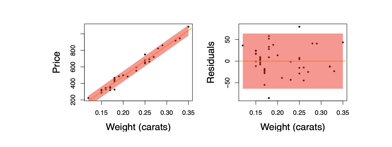
- The variability of points around the least squares line should be roughly constant.
- This implies that the variability of residuals around the 0 line should be roughly constant as well.
- Also called homoscedasticity.
Checking for nomality
We can use histogram、Q-Q plot and Jarque–Bera test to check the normality assumption.
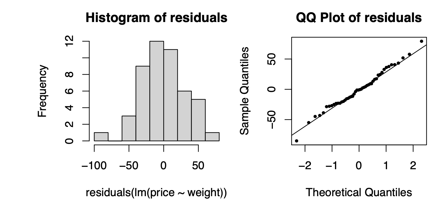
- The residual histogram is consistent with the normality assumption.
- Q-Q plot: The points stay close to the line, suggesting normality.
- Jarque–Bera test: to test whether sample data have the skewness and kurtosis matching a normal distribution.
Histogram
1
2
3
4
5
6
7
8
9
10
11
12
13
14
15
16
17
18
19
20
21
22
23
24
25
26
27
28
29
30
# Histogram with 30 bins;
df.hist(bins=30)
# it can return the number for each bin;

"""
Returns
    -------
    n : array or list of arrays
        The values of the histogram bins. See *density* and *weights* for a
        description of the possible semantics.  If input *x* is an array,
        then this is an array of length *nbins*. If input is a sequence of
        arrays ``[data1, data2, ...]``, then this is a list of arrays with
        the values of the histograms for each of the arrays in the same
        order.  The dtype of the array *n* (or of its element arrays) will
        always be float even if no weighting or normalization is used.

    bins : array
        The edges of the bins. Length nbins + 1 (nbins left edges and right
        edge of last bin).  Always a single array even when multiple data
        sets are passed in.

    patches : `.BarContainer` or list of a single `.Polygon` or list of such objects
        Container of individual artists used to create the histogram
        or list of such containers if there are multiple input datasets.


"""
#For more help, use:
import matplotlib.pyplot as plt
help(plt.hist)
Q-Q plot
1
2
3
4
5
6
7
8
import numpy as np
import statsmodels.api as sm
from matplotlib import pyplot as plt

data_points = np.random.normal(0, 1, 100)
sm.qqplot(data_points, line ='s')
plt.show()
Jarque–Bera test
In statistics, the Jarque–Bera test is a goodness-of-fit test of whether sample data have the skewness and kurtosis matching a normal distribution. The test is named after Carlos Jarque and Anil K. Bera. The test statistic is always nonnegative. If it is far from zero, it signals the data do not have a normal distribution.
If the data comes from a normal distribution, the JB statistic asymptotically has a chi-squared distribution with two degrees of freedom, so the statistic can be used to test the hypothesis that the data are from a normal distribution. The null hypothesis is a joint hypothesis of the skewness being zero and the excess kurtosis being zero. Samples from a normal distribution have an expected skewness of 0 and an expected excess kurtosis of 0 (which is the same as a kurtosis of 3). As the definition of JB shows, any deviation from this increases the JB statistic.
 Meandering pattern shows that the residuals violate the independence assumption, i.e. auto-correlated
 Because the residuals fan out as the # of crews increases, these data violate the assumption of equal error variance in the model.
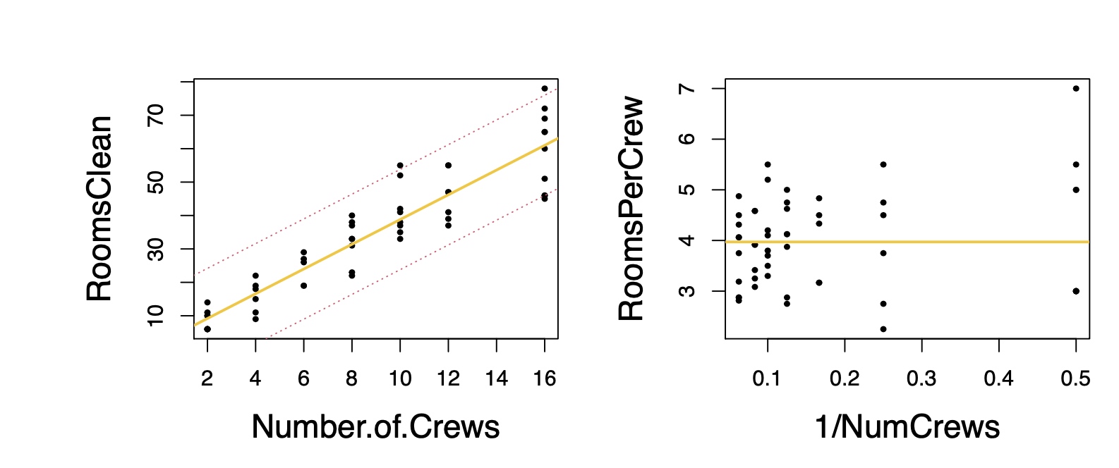
- Over and under estimate variance for different x region
- Consider RoomsClean per Crew as y
Outliers
- Outliers are points that lie away from the cloud of points.
- High leverage points: outliers that lie horizontally away from the center of the cloud.
- Influential points: high leverage points that actually influence the slope of the regression line.
- In order to determine if a point is influential, visualize the regression line with and without the point. Does the slope of the line change considerably?
- If so, then the point is influential.
- If not, then it’s not an influential point.

- Leverage points can impact inferences in dramatic fashion.
- The data cottages.dat contains the profits obtained by a construction firm for 18 properties, as well as the square footage of each of the properties.

Relevant Questions
Q1: Is $\beta_1$ = 0? i.e. is X an important variable?
- We use a hypothesis test to answer this question.
Q2: Confidence Interval for β1
We not only care about whether β1 = 0, but also what exact values β1 takes. We can calculate confidence interval for β1 using the same idea as for μ.
Q3: Confidence Interval for E(y |x)
\[E(y\vert x) = \beta_0 + \beta_1x\]What is the average price for all rings with 1/4 carat diamonds?
 Q4: Prediction Interval for y
How much might pay for a specific ring with a 1/4 carat diamond?
 Q5: Interpretation of RMSE
Root Mean Squared Error (RMSE):
\[M S E=\frac{S S E}{n-2} \quad R M S E=\sqrt{M S E}\]- RMSE tells us how far our predictions are off on average.
- Drawback: RMSE depends on the size of Y .
- Example: diamond price in RMB vs Singapore dollors.
RMSE is especially important in regression. If the simple linear regression model holds, i.e.
- Linear relationship
- Independence among the residuals
- The residuals have constant variance
- Normally distributed residuals
then we have the following approximations:
- 68% of the observed y will lie within 1×RMSE of the predicted y
- 95% of the observed y will lie within 2×RMSE of the predicted y
- 99.7% of the observed y will lie within 3×RMSE of the predicted y
Estimating the parameters
\[\mathrm{RSS}=\sum_{i=1}^{n} \varepsilon_{i}^{2}=\sum_{i=1}^{n}\left(y_{i}-\alpha-\beta x_{i}\right)^{2}\]where RSS is the commonly used acronym for the residual sum of squares (sum of squared residuals would probably be a more accurate description, but RSS is the convention).
With the framework of OLS, in order to minimize this equation, we first take its derivative with respect to $\alpha $ and $\beta$ separately.
We set the derivatives to zero and solve the resulting simultaneous equations. The result is the equations for OLS parameters:
\[\alpha=\bar{Y}-\beta \bar{X}\] \[\beta=\frac{\sum_{i=1}^{n} x_{i} y_{i}-n \bar{Y} \bar{X}}{\sum_{i=1}^{n} x_{i}^{2}-n \bar{X}^{2}}\]where $\bar{X}$ and $\bar{Y}$ are the sample mean of X and Y, respectively.
Evaluating the regression
Evaluation: R square
In finance it is rare that a simple univariate regression model is going to completely explain a large data set. In many cases, the data are so noisy that we must ask ourselves if the model is explaining anything at all. Even when a relationship appears to exist, we are likely to want some quantitative measure of just how strong that relationship is.
Probably the most popular statistic for describing linear regressions is the coefficient of determination, commonly known as R-squared, or just $R^2$.
To calculate the coefficient of determination, we need to define two additional terms: the total sum of squares (TSS) and the explained sum of squares (ESS). They are defined as:
\[\mathrm{TSS}=\sum_{i=1}^{n}\left(y_{i}-\bar{Y}\right)^{2}\] \[\mathrm{ESS}=\sum_{i=1}^{n}\left(\hat{y}_{i}-\bar{Y}\right)^{2}=\sum_{i=1}^{n}\left(\alpha+\beta x_{i}-\bar{Y}\right)^{2}\]These two sums are related to the previously encountered residual sum of squares, as follows:
\[TSS=RSS+ESS\]These sums can be used to compute $R^2$:
\[R^2=\frac{ESS}{TSS}=1-\frac{RSS}{TSS}\]As promised, when there are no residual errors, when RSS is zero, $R^2$ is one. Also, when ESS is zero, or when the variation in the errors is equal to TSS, $R^2$ is zero.
It turns out that for the univariate linear regression model, R2 is also equal to the correlation between X and Y, squared.
\[R^2=\frac{Var(\alpha +\beta X)}{Var(Y)}\]since we know that:
\[Var(\alpha +\beta X)=\beta^2 \sigma_X^2\]and
\[\beta=\rho(X,Y) \frac{\sigma_Y}{\sigma_X}\]we have
\[R^2= \rho^2(X,Y)\]Evaluation: Significance of the parameters
In regression analysis, the most common null hypothesis is that the slope parameter, $\beta$, is zero. If $\beta$ is zero, then the regression model does not explain any variation in the regressand.
In finance, we often want to know if $\alpha$ is significantly different from zero, but for different reasons. In modern finance, alpha has become synonymous with the ability of a portfolio manager to generate excess returns.
In order to test the significance of the regression parameters, we first need to calculate the variance of α and β, which we can obtain from the following formulas:
\[\hat{\sigma}_{\varepsilon}^{2}=\frac{\sum_{i=1}^{n} \varepsilon_i^2}{n-2}\] \[\hat{\sigma}_{\alpha}^{2}=\frac{\sum_{i=1}^{n} x_{i}^{2}}{n \sum_{i=1}^{n}\left(x_{i}-\bar{x}\right)^{2}} \hat{\sigma}_{\varepsilon}^{2}\] \[\hat{\sigma}_{\beta}^{2}=\frac{\hat{\sigma}_{\varepsilon}^{2}}{ \sum_{i=1}^{n}\left(x_{i}-\bar{x}\right)^{2}}\]Proof:
The first formula gives the variance of the error term, $\varepsilon$, which is simply the RSS divided by the degrees of freedom for the regression (T-n).
\[\hat{\beta}=\frac{\sum(X_i -\bar{X})(Y_i-\bar{Y})}{\sum (X_i-\bar{X})^2}\]since
\[Y_i=\alpha + \beta X_i +\varepsilon_i\] \[\bar{Y}=\alpha + \beta \bar{X}\]we have
\[Y_i-\bar{Y}=\beta (X_i-\bar{X}) + \varepsilon_i\]Plug in the original equation, we have:
\[\hat{\beta}=\frac{\sum(X_i -\bar{X})(\beta (X_i-\bar{X}) + \varepsilon_i)}{\sum (X_i-\bar{X})^2}=\beta+\frac{\sum(X_i -\bar{X})\varepsilon_i}{\sum (X_i-\bar{X})^2}\]As a result, we have
\[V(\hat{\beta})=V(\varepsilon) \frac{\sum(X_i -\bar{X})^2}{(\sum (X_i-\bar{X})^2)^2}=\frac{V(\varepsilon)}{\sum (X_i-\bar{X})^2}\]For $\hat{\alpha}$:
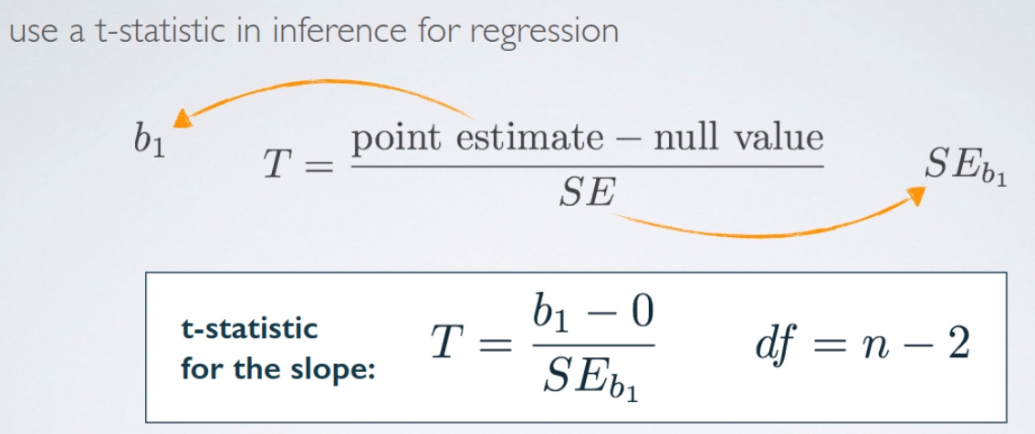
\[\begin{aligned} \hat{\alpha}&= \bar{Y}-\hat{\beta} \bar{X} \\ &= \bar{Y}-\hat{\beta} \sum \frac{X_i}{n} \end{aligned}\]Using the equations for the variance of our estimators, we can then form an appropriate t-statistic. For example, for $\beta$ we would have
\[\frac{\hat{\beta}-\beta}{\hat{\sigma}_{\beta}} \sim t_{n-2}\]The most common null hypothesis when testing regression parameters is that the parameters are equal to zero. More often than not, we do not care if the parameters are significantly greater than or less than zero; we just care that they are significantly different than 0. Because of this, rather than using the standard t-statistics as in Equation 10.17, some practitioners prefer to use the absolute value of the t-statistic. Some software packages also follow this convention.
Linear regression (Multivariate)
\[Y=X\beta + \varepsilon\]No Multicollinearity/Collinearity
In the multivariate case, we require that all of the independent variables be linearly independent of each other. We say that the independent variables must lack multicollinearity:
A7: The independent variables have no multicollinearity.
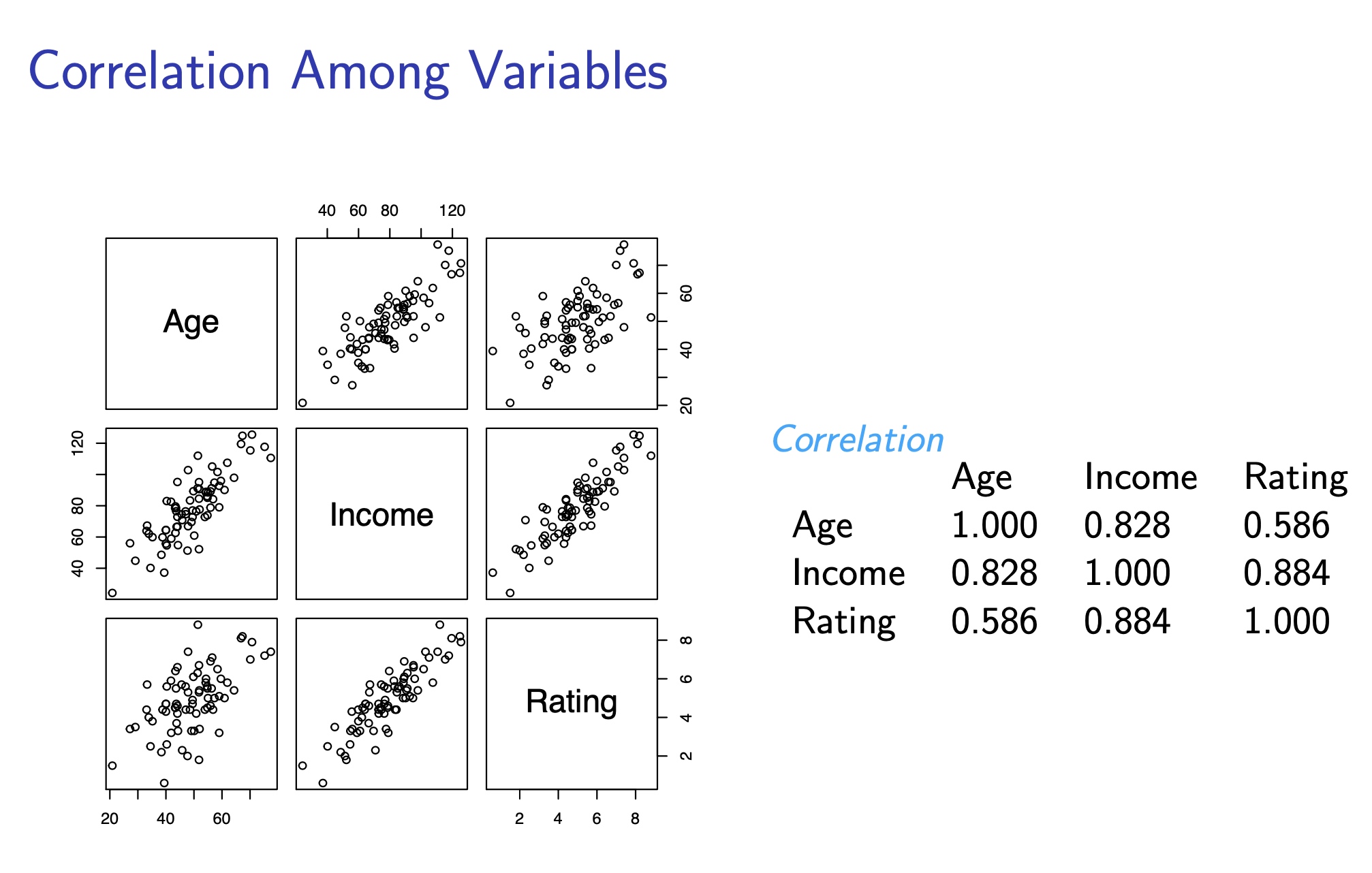
MRM allows the use of correlated explanatory variables. Collinearity occurs when the correlations among the X variables are large. As the correlation among these variables grows, it becomes difficult for regression to separate the partial effects of different variables.
- Highly correlated X variables tend to change together, making it difficult to estimate the partial slope.
- Difficulties interpreting the model
There is no well-accepted procedure for dealing with multicollinearity.
1) eliminate a variable The easiest course of action is often simply to eliminate a variable from the regression. While easy, this is hardly satisfactory.
2) transform the variables Another possibility is to transform the variables, to create uncorrelated variables out of linear combinations of the existing variables. In the previous example, even though $X_3$ is correlated with $X_2$, $X_3-\lambda X_2$ is uncorrelated with $X_2$.
3) PCA
One potential problem with this approach is similar to what we saw with principal component analysis (which is really just another method for creating uncorrelated variables from linear combinations of correlated variables).
Make economic sense?
If we are lucky, a linear combination of variables will have a simple economic interpretation. For example, if X2 and X3 are two equity indexes, then their difference might correspond to a familiar spread. Similarly, if the two variables are interest rates, their difference might bear some relation to the shape of the yield curve. Other linear combinations might be difficult to interpret, and if the relationship is not readily identifiable, then the relationship is more likely to be unstable or spurious.


Discussion: The F Test and Correlated Predictors
- Seemingly contradiction between
- Overall F Ratio in the ANOVA Table
- Individual p-value (T test) for each regression coefficient
- The overall F Ratio comes in handy when the explanatory variables in a regression are correlated.
- Overall F Ratio: whether at least one of the X variables is significant, leaving out the other ones
- Individual T test: whether each individual X variable is significant, having included the other ones
- When the predictors are highly correlated (i.e. high collinearity), they may contradict each other.
Measuring Collinearity: Variance Inflation Factor (VIF)
- The lower VIF is, the less collinearity.
- The VIF is the ratio of the variation that was originally in each explanatory variable to the variation that remains after removing the effects of the other explanatory variables.
- If the x’s are uncorrelated, VIF = 1.
- If the x’s are correlated, VIF can be much larger than 1.
The VIF answers a very handy question when an explanatory variable is not statistically significant: Is this explanatory variable simply not useful, or is it just redundant?
Summary for Collinearity
- Collinearity is the presence of “substantial” correlation among the explanatory variables (the X’s) in a multiple regression.
- Potential redundancy among the X’s
- The F Ratio detects statistical significance that can be disguised by collinearity.
- The F ratio allows you to look at the importance of several factors simultaneously.
- When predictors are collinear, the F test reveals their net effect, rather than trying to separate their effects as a t ratio does.
- VIF measures the impact of collinearity on the coefficients of specific explanatory variables.
Estimating the parameters
The result is our OLS estimator for $\beta $, $\hat{\beta}$:
\[\hat{\boldsymbol{\beta}}=\left(\mathbf{X}^{\prime} \mathbf{X}\right)^{-1} \mathbf{X}^{\prime} \mathbf{Y}\]Where we had two parameters in the univariate case, now we have a vector of n parameters, which define our regression equation.
Given the OLS assumptions—actually, we don’t even need assumption A6, that the regressors are nonstochastic— $\hat{\beta}$ is the best linear unbiased estimator of $\beta$. This result is known as the Gauss-Markov theorem.
Evaluation of the regression
Evaluation: R square and adjusted R square
One problem in the multivariate setting is that $R^2$ tends to increase as we add independent variables to our regression.
Clearly there should be some penalty for adding variables to a regression. An attempt to rectify this situation is the adjusted $R^2$, which is typically denoted by $R^2$, and defined as:
\[\bar{R}^{2}=1-\left(1-R^{2}\right) \frac{t-1}{t-n}\]where t is the number of sample points and n is the number of regressors, including the constant term.
Evaluation: significance of parameters with t-statistics
Just as with the univariate model, we can calculate the variance of the error term. Given t data points and n regressors, the variance of the error term is:
\[\hat{\sigma}_{\varepsilon}^{2}=\frac{\sum_{i=1}^{t} \varepsilon_{i}^{2}}{t-n}\]The variance of the i-th estimator is then:
\[\hat{\sigma}_{i}^{2}=\hat{\sigma}_{\varepsilon}^{2}\left[\left(\mathbf{X}^{\prime} \mathbf{X}\right)^{-1}\right]_{i, i}\]Proof
If A=A’ and A is invertible, we know that
\[(A^{-1})'=(A')^{-1}\]Therefore:
\[((X'X)^{-1})'=(X'X)^{-1}\]The inverse of a symmetric matrix is still symmetric.
For the BLUE $\hat{\beta}$, we have:
\[\begin{aligned} \hat{\beta}&=(X'X)^{-1}X'Y\\ &=(X'X)^{-1}X'(X\beta +\varepsilon)\\ &=\beta + (X'X)^{-1}X'\varepsilon \end{aligned}\]For a random variable $X\in R^{n\times 1}$, the covariance matrix can be expressed as:
\[Var(X)=E(X*X')-E(X)*E(X')\]Remember that, for some random vector $X$ and some non-random matrix $A$, we have
\[Var(AX)=A*Var(X)*A'\]we have:
\[V(\hat{\beta})=(X'X)^{-1}X' V(\varepsilon)X(X'X)^{-1}\]Since $V(\varepsilon)=\sigma_{\varepsilon}^2 I$
\[V(\hat{\beta})=\sigma_{\varepsilon}^2 (X'X)^{-1}X' X(X'X)^{-1}=\sigma_{\varepsilon}^2 (X'X)^{-1}\]Therefore, the variance of the i-th estimator is
\[\hat{\sigma}_{i}^{2}=\hat{\sigma}_{\varepsilon}^{2}\left[\left(\mathbf{X}^{\prime} \mathbf{X}\right)^{-1}\right]_{i, i}\]We can then use this to form an appropriate t-statistic, with t −n degrees of freedom:
\[\frac{\hat{\beta}_{i}-\beta_{i}}{\hat{\sigma}_{i}} \sim t_{t-n}\]Evaluation: significance of parameters with F-statistics
Is At Least One $\beta_k \neq 0$?
Instead of just testing one parameter, we can actually test the significance of all of the parameters, excluding the constant, using what is known as an F-test. The F-statistic can be calculated using $R^2$:
\[\frac{ESS/(n-1)}{RSS/(t-n)}=\frac{R^{2} /(n-1)}{\left(1-R^{2}\right) /(t-n)} \sim F_{n-1, t-n}\]- The ANOVA table supplies a highly significant F-ratio.
- This model explains statistically significant variation in Y .
- Atleast one $\beta_k$ is not zero, i.e. at least one of the $X_k $ is useful in predicting Y .
- The ANOVA Table allows you to look at the importance of several factors simultaneously.
SRM of Rating, one variable at a time
\[\begin{array}{lllll} \hline & \text { Estimate } & \text { Std. Error } & t \text { value } & \operatorname{Pr}(>|t|) \\ \hline \text { (Intercept) } & 0.49004 & 0.73414 & 0.668 & 0.507 \\ \text { Age } & 0.09002 & 0.01456 & 6.181 & 3.3 \mathrm{e}-08 \\ \hline \hline & \text { Estimate } & \text { Std. Error } & t \text { value } & \operatorname{Pr}(>|t|) \\ \hline \text { (Intercept) } & -0.598441 & 0.354155 & -1.69 & 0.0953 \\ \text { Income } & 0.070039 & 0.004344 & 16.12 & <2 e-16 \\ \hline \end{array}\]MRM of Rating, on both variables
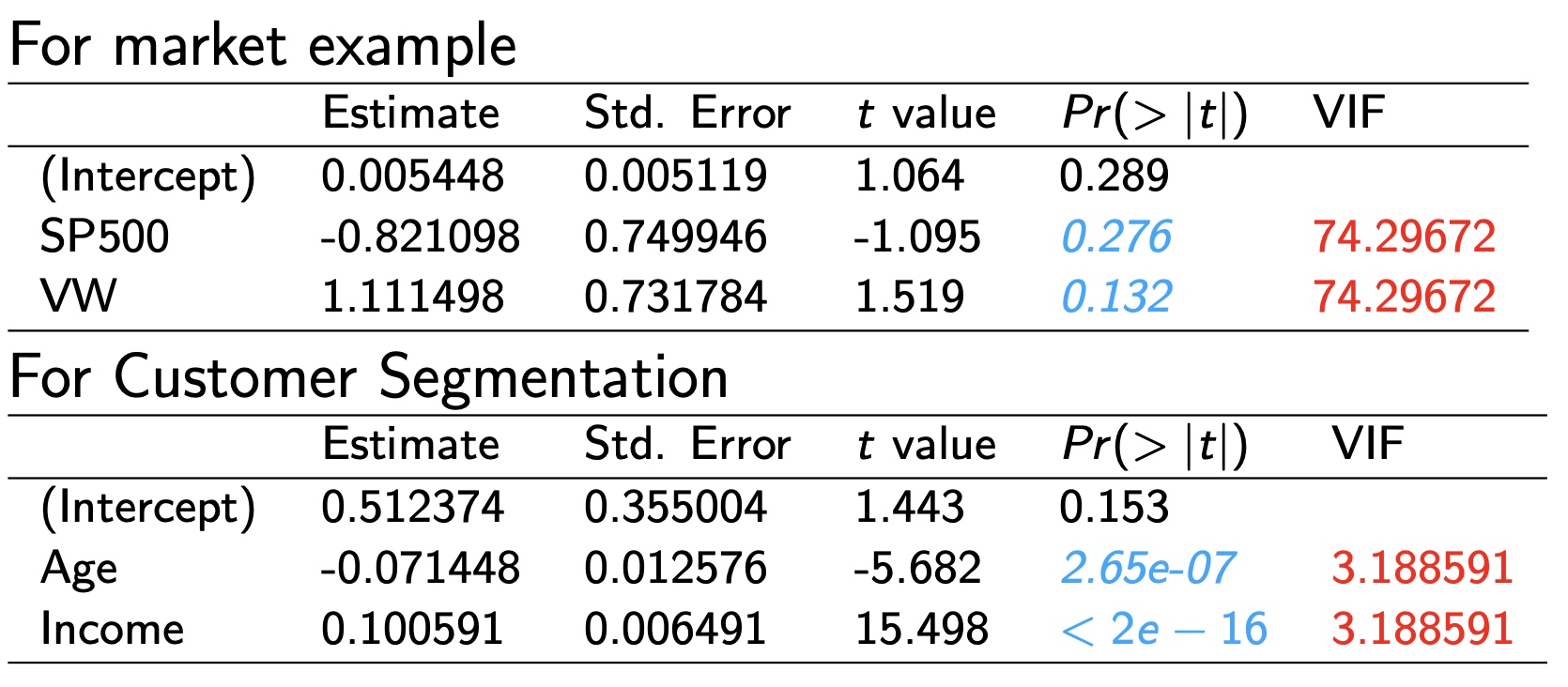
\[\begin{array}{lllll} \hline & \text { Estimate } & \text { Std. Error } & t \text { value } & \operatorname{Pr}(>|t|) \\ \hline \text { (Intercept) } & 0.512374 & 0.355004 & 1.443 & 0.153 \\ \text { Age } & -0.071448 & 0.012576 & -5.682 & 2.65 \mathrm{e}-07 \\ \text { Income } & 0.100591 & 0.006491 & 15.498 & <2 e-16 \end{array}\]We can divide the customer into 3 segments:
- low incomes (< 45K),
- moderate incomes (70K ∼ 80K),
- high incomes (> 110K).
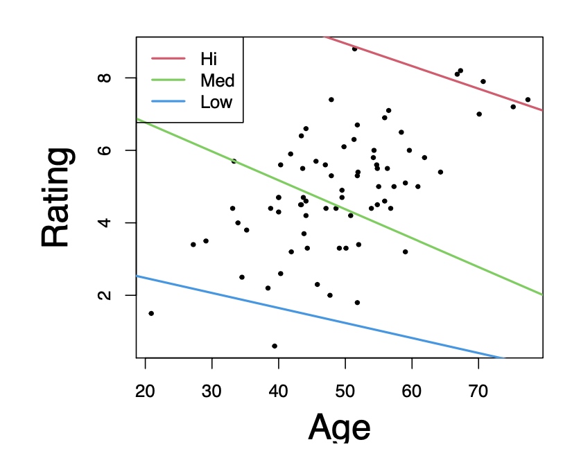
Low income
\[\begin{array}{lllll} \hline & \text { Estimate } & \text { Std. Error } & t \text { value } & \operatorname{Pr}(>|t|) \\ \hline \text { (Intercept) } & 3.30845 & 3.42190 & 0.967 & 0.436 \\ \text { Age } & -0.04144 & 0.10786 & -0.384 & 0.738 \\ \hline \end{array}\]Moderate incomes
\[\begin{array}{lllll} \hline & \text { Estimate } & \text { Std. Error } & t \text { value } & \operatorname{Pr}(>|t|) \\ \hline \text { (Intercept) } & 8.36412 & 2.34772 & 3.563 & 0.0026 \\ \text { Age } & -0.07978 & 0.04791 & -1.665 & 0.1153 \\ \hline \end{array}\]High income
\[\begin{array}{lllll} \hline & \text { Estimate } & \text { Std. Error } & t \text { value } & \operatorname{Pr}(>|t|) \\ \hline \text { (Intercept) } & 12.07081 & 1.28999 & 9.357 & 0.000235 \\ \text { Age } & -0.06243 & 0.01873 & -3.332 & 0.020727 \\ \hline \end{array}\]The simple regression slopes are negative in each case, as in the multiple linear regression.
In general, we want to keep our models as simple as possible. We don’t want to add variables just for the sake of adding variables. This principle is known as parsimony.
$\bar{R}^2$ , t-tests, and F-tests are often used in deciding whether to include an additional variable in a regression.
In finance, even when the statistical significance of the betas is high, $R^2$ and $\bar{R}^2$ are often very low. For this reason, it is common to evaluate the addition of a variable on the basis of its t-statistic. If the t-statistic of the additional variable is statistically significant, then it is kept in the model. It is less common, but it is possible to have a collection of variables, none of which are statistically significant by themselves, but which are jointly significant. This is why it is important to monitor the F-statistic as well.
When applied systematically, this process of adding or remov ing variables from a regression model is referred to as stepwise regression.
Application of linear regression
Application: Factor analysis
In a large, complex portfolio, it is sometimes far from obvious how much exposure a portfolio has to a given factor. Depending on a portfolio manager’s objectives, it may be desirable to minimize certain factor exposures or to keep the amount of risk from certain factors within a given range. It typically falls to risk management to ensure that the factor exposures are maintained at acceptable levels.
The classic approach to factor analysis can best be described as risk taxonomy.
These kinds of obvious questions led to the development of various statistical approaches to factor analysis. One very popular approach is to associate each factor with an index, and then to use that index in a regression analysis to measure a portfolio’s exposure to that factor.
\[r_{\text {portfolio }}=\alpha+\beta r_{\text {index }}+\varepsilon\]Another nice thing about factor analysis is that the factor exposures can be added across portfolios.
\[r_{\mathrm{A}}=\alpha_{\mathrm{A}}+\beta_{\mathrm{A}} r_{\text {index }}+\varepsilon_{\mathrm{A}}\] \[r_{\mathrm{B}}=\alpha_{\mathrm{B}}+\beta_{\mathrm{B}} r_{\text {index }}+\varepsilon_{\mathrm{B}}\] \[r_{\mathrm{A}+\mathrm{B}}=\left(\alpha_{\mathrm{A}}+\alpha_{\mathrm{B}}\right)+\left(\beta_{\mathrm{A}}+\beta_{\mathrm{B}}\right) r_{\text {index }}+\left(\varepsilon_{\mathrm{A}}+\varepsilon_{\mathrm{B}}\right)\]In addition to giving us the factor exposure, the factor analysis allows us to divide the risk of a portfolio into systematic and idiosyncratic components.
\[\sigma_{\text {portfolio }}^{2}=\beta^{2} \sigma_{\text {index }}^{2}+\sigma_{\varepsilon}^{2}\]In theory, factors can be based on almost any kind of return series. The advantage of indexes based on publicly traded securities is that it makes hedging very straightforward.
At the same time, there might be some risks that are not captured by any publicly traded index. Some risk managers have attempted to resolve this problem by using statistical techniques, such as principal component analysis (PCA) or cluster analysis, to develop more robust factors.
Application: Stress Testing
In risk management, stress testing assesses the likely impact of an extreme, but plausible, scenario on a portfolio. There is no universally accepted method for perform- ing stress tests. One popular approach, which we consider here, is closely related to factor analysis.
The first step in stress testing is defining a scenario. Scenarios can be either ad hoc or based on a historical episode.
In the second step, we need to define how all other underlying financial instruments react, given our scenario. In order to do this, we construct multivariate regressions. We regress the returns of each underlying financial instrument against the returns of the instruments that define our scenario.
What might seem strange is that, even in the case of the historical scenarios, we use recent returns in our regression. In the case of the historical scenarios, why don’t we just use the actual returns from that period?
- some securities or companies may not exist
- the relationship between variables has changed significantly
In the final step, after we have generated the returns for all of the underlying financial instruments, we price any options or other derivatives. While using delta approximations might have been acceptable for calculating value at risk statistics at one point in time, it should never have been acceptable for stress testing. By definition, stress testing is the examination of extreme events, and the accurate pricing of nonlinear instruments is critical.
Chapter 8: Time Series Models
Time series describe how random variables evolve over time and form the basis of many financial models.
Random Walks
For a random variable X, with a realization $X_t$ at time t, the following conditions describe a random walk:
\[\begin{aligned} x_{t} &=x_{t-1}+\varepsilon_{t} \\ E\left[\varepsilon_{t}\right] &=0 \\ E\left[\varepsilon_{t}^{2}\right] &=\sigma^{2} \\ E\left[\varepsilon_{s} \varepsilon_{t}\right] &=0 ~~\forall s \neq t \end{aligned}\]By definition, we can see how the equation evolves over multiple periods:
\[x_t=x_{t-1} + \varepsilon_t =x_{t-2}+ \varepsilon_{t}+ \varepsilon_{t-1} =x_0 +\sum_{i=1}^t \varepsilon_i\]Using this formula, it is easy to calculate the conditional mean and variance of $x_t$:
\[\begin{aligned} E\left[x_{t} \mid x_{0}\right] &=x_{0} \\ \operatorname{Var}\left[x_{t} \mid x_{0}\right] &=t \sigma^{2} \end{aligned}\]For a random walk, our best guess for the future value of the variable is simply the current value, but the probability of finding it near the current value becomes increasingly small.
For a random walk, skewness is proportional to $t^{-0.5}$, and kurtosis is proportional to $t^{-1}$.
Drift-Diffusion Model
The simple random walk is not a great model for equities, where we expect prices to increase over time, or for interest rates, which cannot be negative. With some rather trivial modification, though, we can accommodate both of these requirements.
One simple modification we can make to the random walk is to add a constant term, in the following way:
\[p_t=\alpha + p_{t-1} + \varepsilon_t\]Just as before, the variance of $ \varepsilon_t$ is constant over time, and the various $ \varepsilon_t$’s are uncorrelated with each other.
The choice of pt for our random variable is intentional. If $p_t$ is the log price, then rearranging terms, we obtain an equation for the log return:
\[r_t=\Delta p_t = \alpha +\varepsilon_t\]The constant term, $\alpha$, is often referred to as the drift term, for reasons that will become apparent. In these cases, $\varepsilon_t$ is typically referred to as the diffusion term.
Putting these two terms together, the entire equation is known as a drift-diffusion model.
When equity returns follow a drift-diffusion process, we say that equity markets are perfectly efficient. We say they are efficient because the return is impossible to forecast based on past prices or returns. Put another way, the conditional and unconditional returns are equal. Mathematically:
\[E[r_t \mid r_{t-1}]=E[r_t]=\alpha\]As with the random walk equation, we can iteratively substitute the drift-diffusion model into itself:
\[p_{t}=2 \alpha+p_{t-2}+\varepsilon_{t}+\varepsilon_{t-1}=t \alpha+p_{0}+\sum_{i=1}^{t} \varepsilon_{i}\]And just as before, we can calculate the conditional mean and variance of our drift-diffusion model:
\[\begin{aligned} E[p_t \mid p_{t-1}]&=p_0 +t\alpha \\ Var[p_t \mid p_{t-1}]&=t\sigma^2 \end{aligned}\]Autoregression
The next modification we’ll make to our time series model is to multiply the lagged term by a constant:
\[r_t=\alpha +\lambda r_{t_1}+\varepsilon_t\]The equation above is known as an autoregressive (AR) model. More specifically, it is known as an AR(1) model, since $r_t$ depends only on its first lag. The random walk is then just a special case of the AR(1) model, where $\alpha$ is zero and $\lambda $ is equal to one. Although our main focus will be on AR(1) models, we can easily construct an AR(n) model as follows:
\[r_{t}=\alpha+\lambda_{1} r_{t-1}+\lambda_{2} r_{t-2}+\cdots+\lambda_{n} r_{t-n}+\varepsilon_{t}\]We can iteratively substitute our AR(1) model into itself to obtain the following equation:
\[r_{t}=\alpha \sum_{i=0}^{n-1} \lambda^{i}+\lambda^{n} r_{t-n}+\sum_{i=0}^{n-1} \lambda^{i} \varepsilon_{t-i}\]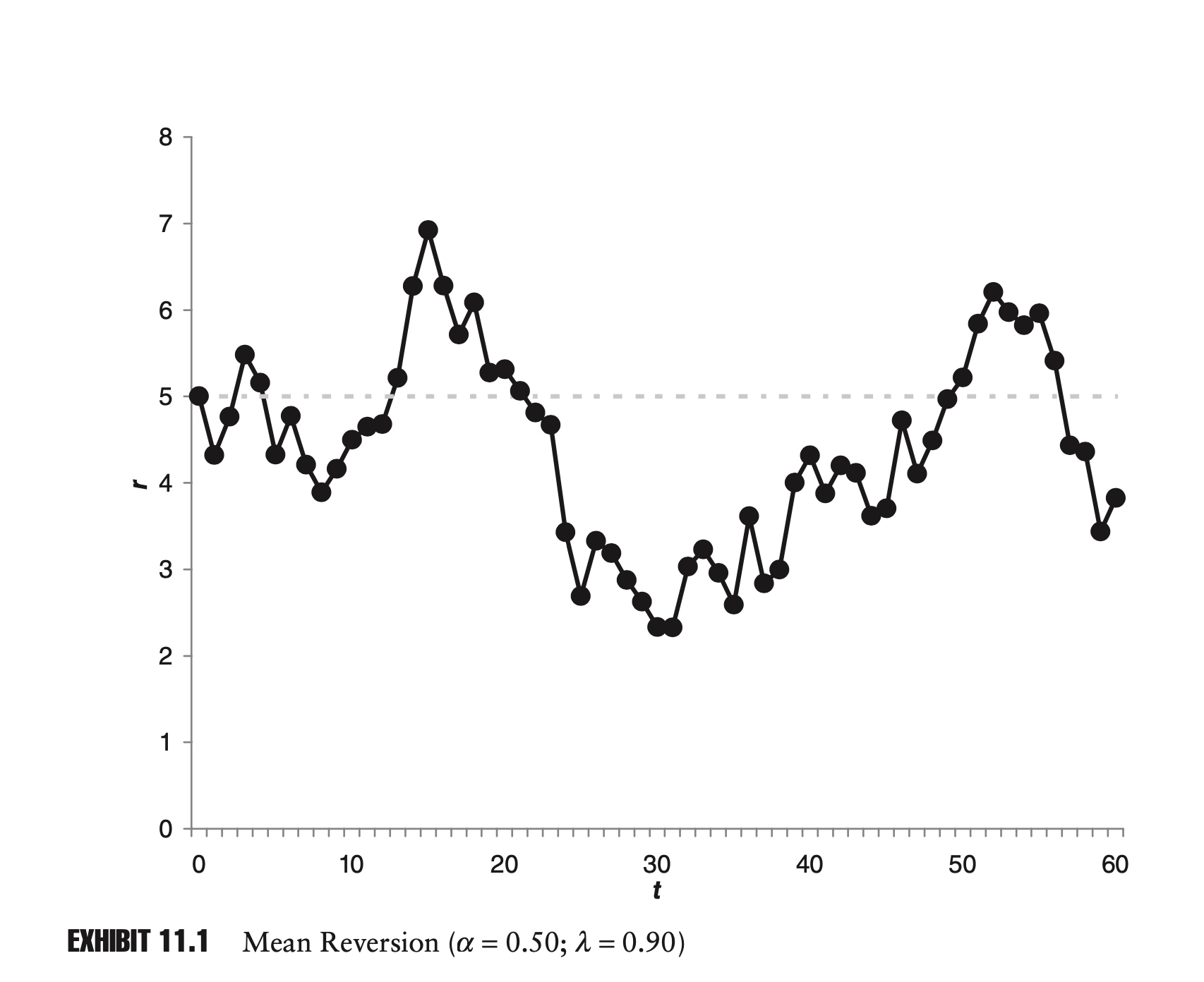

Propositions for AR(1) model
\[r_t=\alpha +\lambda r_{t-1}+\varepsilon_t\]P1 - the long-term trend: If there exists a long-term limit or trend $r^\star$, it must be
\[r^\star = \frac{\alpha }{1-\lambda}\]P2 - existence of long-term stability: The series has convergence iff $| \lambda |<1$.
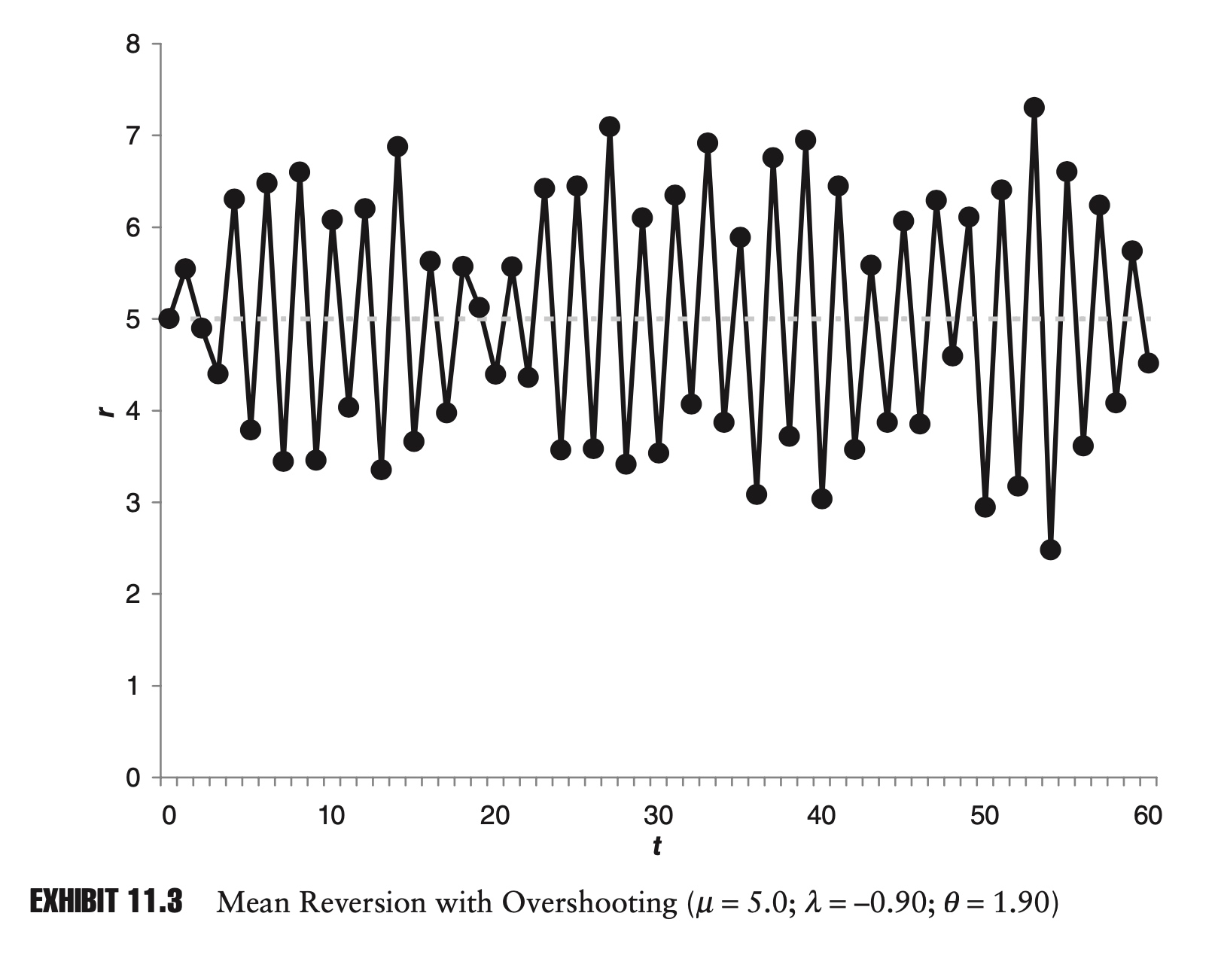
\[r_t-\frac{\alpha }{1-\lambda} =\lambda (r_{t-1}-\frac{\alpha }{1-\lambda})+\varepsilon _t\]P3 - Overshooting
Here overshooting means $r_t - r^\star$ has different sign with $r_{t-1} - r^\star$.
If and only if $\lambda \in (0,1)$, there is no overshooting.
P4 - Linear Combination
\[r_t=\frac{\alpha }{1-\lambda} (1-\lambda ) + \lambda r_{t-1} + \varepsilon _t\]If $\lambda \in (0,1)$, the expectation of $r_t$ is a linear combination of $r^\star$ and $r_{t-1}$. Moreover, $1-\lambda$ is the speed of convergence.
P5 - Mean and Vairance
As mentioned, AR(1) can be expressed as:
\[r_{t}=\alpha \sum_{i=0}^{n-1} \lambda^{i}+\lambda^{n} r_{t-n}+\sum_{i=0}^{n-1} \lambda^{i} \varepsilon_{t-i}\]To proceed further, we can use methods developed in Chapter 1 for summing geometric series. The conditional mean and variance are now:
\[\begin{aligned} E\left[r_{t} \mid r_{t-n}\right] &=\frac{1-\lambda^{n}}{1-\lambda} \alpha+\lambda^{n} r_{t-n} \\ \operatorname{Var}\left[r_{t} \mid r_{t-n}\right] &=\frac{1-\lambda^{2 n}}{1-\lambda^{2}} \sigma^{2} \end{aligned}\]For values of $|\lambda |$ less than one, the AR(1) process is stable. If we continue to ex- tend the series back in time, as n approaches infinity, $\lambda ^n$ becomes increasingly small, causing $\lambda ^n r_{t–n}$ to approach zero. In this case:
\[r_t=\frac{1}{1-\lambda}\alpha + \sum _{i=0}^{\infty} \lambda ^i \varepsilon_{t-i}\]Continuing to use our geometric series techniques, we then arrive at the following results for the mean and variance:
\[\begin{aligned} E[r_t] & = \frac{1}{1-\lambda}\alpha \\ Var[r_t] &=\frac{1}{1-\lambda^2} \sigma^2 \end{aligned}\]So, for values of $|\lambda|$ less than one, as n approaches infinity, the initial state of the system ceases to matter. The mean and variance are only a function of the constants.
P6 - autocorrelation
We can quantify the level of mean reversion by calculating the correlation of $r_t$ with its first lag. This is known as autocorrelation or serial correlation. For our AR(1) series, we have:
\[\rho_{t,t-1}=1-\theta =\lambda\]If $\lambda >0 $, we expect $r_t - r^\star $ tends to have the same sign as $r_{t-1} - r^\star $, and vice versa.
Variance and Autocorrelation
For a random work $r_t=\varepsilon_t$, the n-period return is:
\[y_{n,t}=\sum_{i=0}^{n-1}r_{t-i}=\sum_{i=0}^{n-1} \varepsilon_{t-i}\]As stated before, the variance of $y_{n,t}$ is proportional to n:
\[Var[y_{n,t}]=n\sigma^2_{\varepsilon}\]and the standard deviation of $y_{n,t}$ is proportional to the square root of n.
When we introduce autocorrelation, this square root rule no longer holds.
Instead of a random walk, assume returns follow an AR(1) series:
\[r_{t}=\alpha+\lambda r_{t-1}+\varepsilon_{t}=\frac{\alpha}{1-\lambda}+\sum_{i=0}^{\infty} \lambda^{i} \varepsilon_{t-i}\]Now define a two-period return:
\[y_{2, t}=r_{t}+r_{t-1}=\frac{2 \alpha}{1-\lambda}+\varepsilon_{t}+\sum_{i=0}^{\infty} \lambda^{i}(1+\lambda) \varepsilon_{t-i-1}\]With just two periods, the introduction of autocorrelation has already made the description of our multi-period return noticeably more complicated. The variance of this series is now:
\[Var[y_{2,t}]=\frac{2}{1-\lambda }\sigma^2_{\varepsilon}\]If $\lambda$ is zero, then our time series is equivalent to a random walk and our new variance formula gives the correct answer: that the variance is still proportional to the length of our multiperiod return.
If $\lambda$ is greater than zero, and serial correlation is positive, then the two-period variance will be more than twice as great as the single-period variance.
Time series with slightly positive or negative serial correlation abound in finance. It is a common mistake to assume that variance is linear in time, when in fact it is not. Assuming no serial correlation when it does exist can lead to a serious overestimation or underestimation of risk.
Stationarity
In the preceding section we discussed unstable series whose means and variances tend to grow without bound. There are many series in the real world that tend to grow exponentially—stock market indexes and gross domestic product (GDP), for example—while other series such as interest rates, inflation, and exchange rates typically fluctuate in narrow bands.
This dichotomy, between series that tend to grow without limit and those series that tend to fluctuate around a constant level, is extremely important in statistics. We call series that tend to fluctuate around a constant level stationary time series. In contrast, series that are divergent are known as nonstationary. Determining whether a series is stationary is often the first step in time series analysis.
To be more precise, we say that a random variable X is stationary if for all t and n:
- $E\left[x_{t}\right]=\mu$ and $|\mu|<\infty$
- $\operatorname{Var}[x_{t}]=\sigma^{2}$ and $|\sigma^{2}|<\infty$
- $\operatorname{Cov}[x_{t}, x_{t-n}]=\sigma_n^2, \forall n$
where $\mu$, $\sigma^2$, and \(\sigma_n, n\in \mathcal{Z}^{+}\) are constants. These three conditions state that the mean, variance, and serial correlation should be constant over time. We also require that the mean and variance be finite.
While we can calculate a sample mean or variance for a nonstationary series, these statistics are not very useful. Because the mean and variance are changing, by definition, these sample statistics will not tell us anything about the mean and variance of the distribution in general.
Regression analysis on nonstationary series is likely to be even more meaningless. If a series is nonstationary because its volatility varies over time, then it violates the ordinary least squares (OLS) requirement of homoscedasticity. Even if the variance is constant, but the mean is drifting, any conclusions we might draw about the relationship between two nonstationary series will almost certainly be spurious.
Example of nonstationary time series analyis
As an example of this type of spurious correlation, imagine two AR(1) series with nonzero drifts. To make the calculations easier, we also assume that both series start at zero:
\[\begin{array}{ll}p_{t}=\alpha_{p}+p_{t-1}+\varepsilon_{p, t} & \text { where } \quad \alpha_{p} \neq 0, p_{0}=0 \\ q_{t}=\alpha_{q}+q_{t-1}+\varepsilon_{q, t} & \text { where } \quad \alpha_{q} \neq 0, q_{0}=0\end{array}\]We assume that both disturbance terms are mean zero and uncorrelated, and therefore the two series are independent by design. In other words, the two series have no causal relationship.
Imagine that we tried to calculate the correlation of p and q between 0 and t:
\[\tilde{\sigma}_{p, q}=\frac{1}{t+1} \sum_{i=0}^{t} p_{i} q_{i}-E[\tilde{p}] E[\tilde{q}]=\frac{1}{t+1} \sum_{i=0}^{t} p_{i} q_{i}-\alpha_{p} \alpha_{q} \frac{t^{2}}{4}\] \[\beta=\frac{\tilde{\sigma}_{p, q}}{\tilde{\sigma}_{p}^{2}}=\frac{\alpha_{p} \alpha_{q} \frac{t^{2}+2 t}{12}}{\alpha_{p}^{2} \frac{t^{2}+2 t}{12}}=\frac{\alpha_{q}}{\alpha_{p}}\]Though it was a long time in coming, this result is rather intuitive. If αp is twice the value of αq, then at any point in time we will expect p to be twice the value of q.
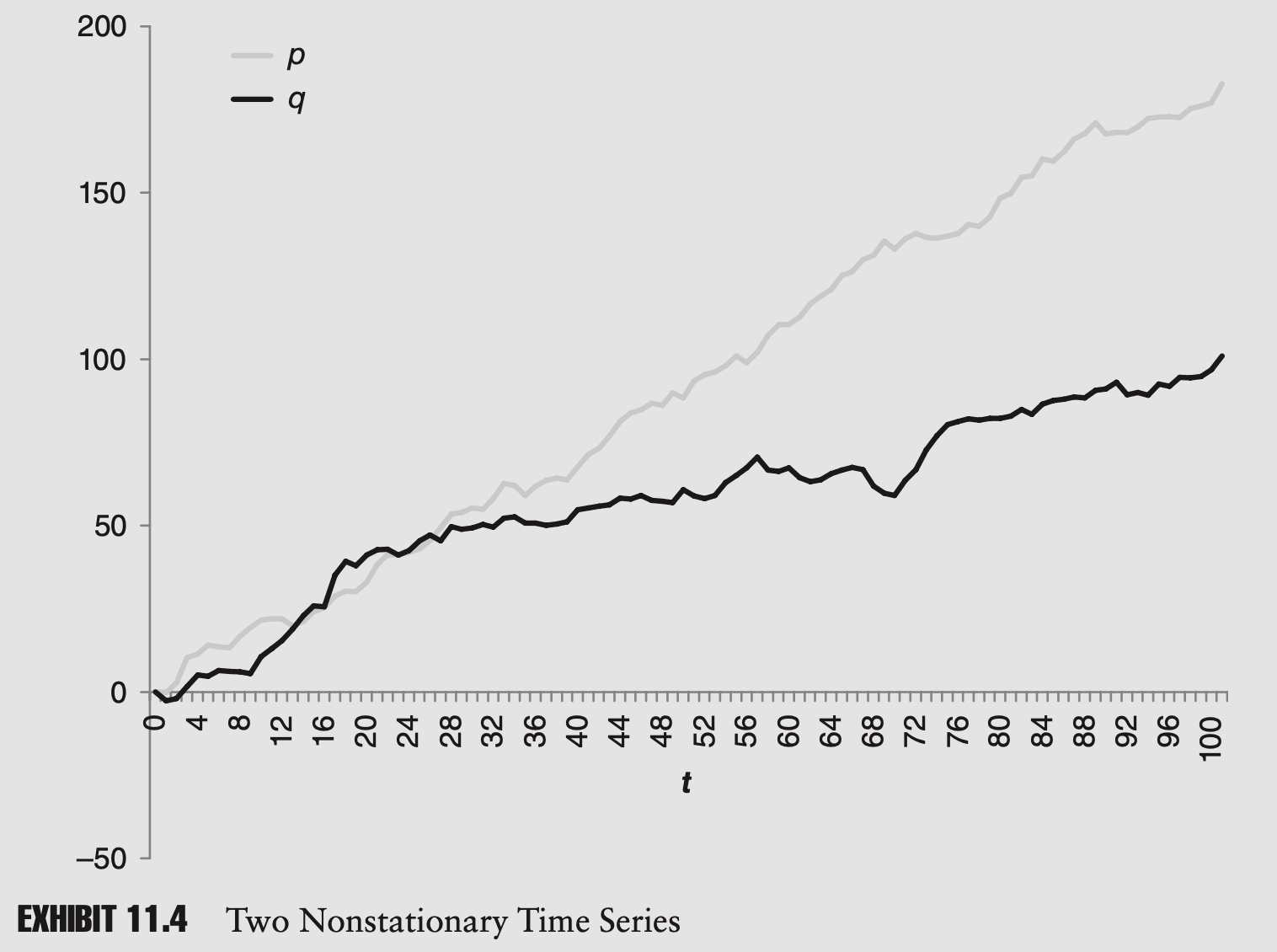
This should all seem very wrong. If two variables are independent, we expect them to have zero covariance, but because these series both have nonzero drift terms, the sample covariance and beta will also tend to be nonzero. The results are clearly spurious.
In a situation such as our sample problem, you could argue that even though the two AR(1) series are independent, the positive sample covariance is telling us something meaningful: that both series have nonzero drift terms. How meaningful is this? Not very, as it turns out. Any random variable with a nonzero mean can be turned into a nonstationary series. Log returns of equities tend to be stationary, but the addition of those returns over time, log prices, are nonstationary.
To show just how silly all of this can get, in a classic example, Hendry (1980) showed how, if statistical analysis is done incorrectly, you might conclude that cumulative rainfall in the United Kingdom and the UK price index where causally related.
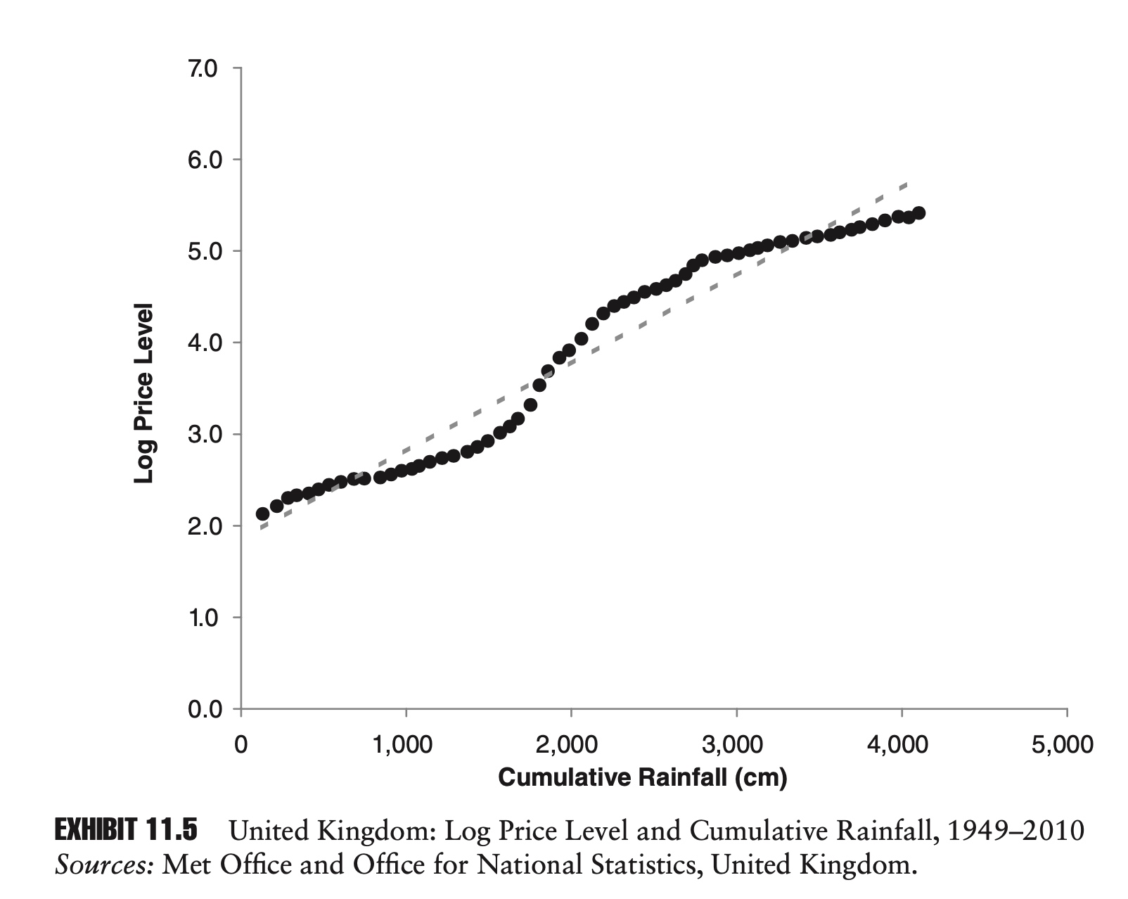
The remedy for stationarity in statistical analysis is clear. Just as we can construct a nonstationary series from a stationary one by summing over time, we can usually create a stationary series from a nonstationary series by taking its difference. Transforming a price series into returns is by now a familiar example. Occasionally additional steps will need to be taken (e.g., differencing twice), but for most financial and economic series, this will suffice.
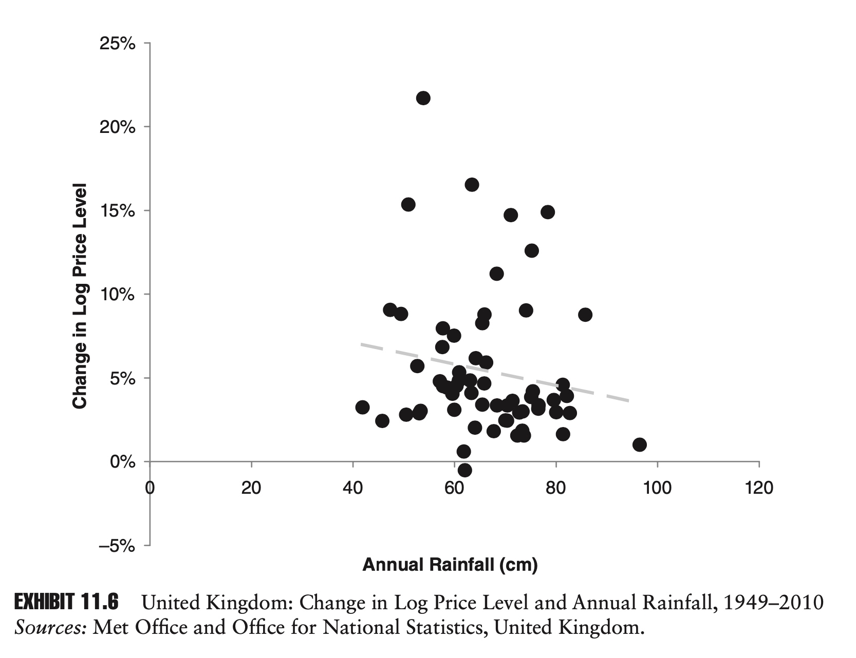
Exhibit 11.6 shows a regression based on the same data set we used in Exhibit 11.5, only now instead of cumulative rainfall we are using annual rainfall, and instead of the log price level we are using changes in the log price index. This new chart looks very different. The regression line is very close to being flat, and the slope parameter is in fact not significant. In other words, rainfall has no meaningful impact on inflation, just as we would expect.
Ascribing a causal relationship when none exists is a serious mistake. Unfortunately, in this day and age, it is easy to gather massive amounts of data and perform a quick regression analysis. When performing statistical analysis of time series data, it is important to check for stationarity.
Moving Average
Besides autoregressive (AR) series, the other major class of time series is moving averages (MAs). An MA(n) series takes the form:
\[x_t=\varepsilon_t + \theta_1 \varepsilon_{t-1}+\theta_2 \varepsilon_{t-2} + \cdots +\theta_n \varepsilon_{t-n}\]Moving average series can be combined with autoregressive series to form ARMA(p,q) processes:
\[x_{t}=\lambda_{1} x_{t-1}+\lambda_{2} x_{t-2}+\cdots+\lambda_{p} x_{t-p}+\varepsilon_{t}+\theta_{1} \varepsilon_{t-1}+\cdots+\theta_{q} \varepsilon_{t-q}\]Moving averages and ARMA processes are important in statistics, but are less common in finance.
Application 1: GARCH
Up until this point, all of our time series models have assumed that the variance of the disturbance term remains constant over time. In financial markets, variance appears to be far from constant. Both prolonged periods of high variance and prolonged periods of low variance are observed.
While the transition from low to high variance can be sudden, more often we observe serial correlation in variance, with gradual mean reversion. When this is the case, periods of above-average variance are more likely to be followed by periods of above-average variance, and periods of below-average variance are likely to be followed by periods of below-average variance.
Exhibit 11.8 shows the rolling annualized 60-day standard deviation of the S&P 500 index between 1928 and 2008. Notice how the level of the standard deviation is far from random. There are periods of sustained high volatility (e.g., 1996–2003) and periods of sustained low volatility (e.g., 1964–1969).

One of the most popular models of time-varying volatility is the autoregressive conditional heteroscedasticity (ARCH) model. We start by defining a disturbance term at time t, $\varepsilon_t$, in terms of an independent and identically distributed (i.i.d.) standard normal variable, $\mu_t$, and a time varying standard deviation, $\sigma_t$:
\[\varepsilon_t= \sigma_t \mu_t\]In the simplest ARCH model, we can model the evolution of the variance as:
\[\sigma_{t}^{2}=\alpha_{0} \bar{\sigma}^{2}+\alpha_{1} \sigma_{t-1}^{2} u_{t-1}^{2}=\alpha_{0} \bar{\sigma}^{2}+\alpha_{1} \varepsilon_{t-1}^{2}\]where $\alpha_0$ and $\alpha_1$ are constants, and $\bar{\sigma}^2$ is the long-run variance. To ensure $\sigma^2$ remains positive, we require $\alpha_0>0$, $\alpha_1>0$, and $\bar{\sigma}^2 > 0$.
For long-run convergence $\bar{\sigma^2} $ to exist, we require that $\alpha_0+ \alpha_1 = 1$.
To prove this, we just have to notice that $\mu_t$ and $\sigma_t$ are independent, and therefore
\[E\left[\sigma_{t-1}^{2} u_{t-1}^{2}\right]=E\left[\sigma_{t-1}^{2}\right] E\left[u_{t-1}^{2}\right]\]Then we have
\[E[\sigma_{t}^{2}]=\alpha_0 \bar{\sigma}^2+ \alpha_1 E[\sigma_{t-1}^{2}]\]Take both side to the limit, we have $\alpha_0+ \alpha_1 = 1$.
The equation above is typically referred to as an ARCH(1) model. By adding more lagged terms containing $\sigma^2$ and $\mu^2$, we can generalize to an ARCH(n) specification:
\[\sigma_t^2=\alpha_0 \bar{\sigma}^2 + \sum_{i=1}^n \alpha_i \sigma_{t-i}^2\mu_{t-i}^2\]Besides the additional disturbance terms, we can also add lags of $\sigma^2$ itself to the equation. In this form, the process is known as generalized autoregressive conditional heteroscedasticity (GARCH). The following describes a GARCH(1,1) process:
\[\sigma_t^2=\alpha_0 \bar{\sigma}^2 + \alpha_1 \sigma_{t-1}^2\mu_{t-1}^2 + \beta \sigma^2_{t-1}\]For the GARCH(1,1) to be stable, we require that $\alpha_0+ \alpha_1 +\beta = 1$. Just as with the ARCH model, by adding additional terms we can build a more general GARCH(n,m) process.
Application 2: Jump-Diffusion Model
In the GARCH model, volatility changes gradually over time. In financial markets we do observe this sort of behavior, but we also see extreme events that seem to come out of nowhere. For example, on February 27, 2007, in the midst of otherwise calm markets, rumors that the Chinese central bank might raise interest rates, along with some bad economic news in the United States, contributed to what, by some measures, was a –8 standard deviation move in U.S. equity markets. A move of this many standard deviations would be extremely rare in most standard parametric distributions.
One popular way to generate this type of extreme return is to add a so-called jump term to our standard time series model. This can be done by adding a second disturbance term:
\[r_t =\alpha +\varepsilon_t + [I_t]\mu_t\]Here, $r_t$ is the market return at time t, $\alpha $ is a constant drift term, and $\varepsilon_t $ is our standard mean zero diffusion term.
As specified, our jump term has two components: $[I_t]$, an indicator variable that is either zero or one, and $u_t$, an additional disturbance term. Not surprisingly, as specified, this time series model is referred to as a jump-diffusion model.
The jump-diffusion model is really just a mixture model. To get the type of behavior we want—moderate volatility punctuated by rare extreme events—we can set the variance of $\varepsilon_t $ to relatively modest levels. We then specify the probability of $[I_t]$ equaling one at some relatively low level, and set the variance of $\mu_t$ at a relatively high level. If we believe that extreme negative returns are more likely than extreme positive returns, we can also make the distribution of ut asymmetrical.
GARCH and jump-diffusion are not mutually exclusive. By combining GARCH and jump-diffusion, we can model and understand a wide range of market environments and dynamics.
Chapter 9: Decay Factors
In this chapter we explore a class of estimators that has become very popular in finance and risk management for analyzing historical data. These models hint at the limitations of the type of analysis that we have explored in previous chapters.
Mean
In previous chapters, we showed that the best linear unbiased estimator (BLUE) for the sample mean of a random variable was given by:
\[\bar{\mu}=\frac{1}{n}\sum_{i=0}^{n-1}x_{t-i}\]For a practitioner, this formula immediately raises the question of what value to use for n. {: .align-center}Should we use 10 years of data? One year? Thirty days? A popular choice in many fields is simply to use all available data. While this can be a sensible approach in some circumstances, it is much less common in modern finance. Using all available data has three potential drawbacks.
First, the amount of available data for different variables may vary dramatically. If we are trying to calculate the mean return for two fixed-income portfolio managers, and we have 20 years of data for one and only two years of data for another, and the last two years have been particularly good years for fixed-income portfolio managers, a direct comparison of the means will naturally favor the manager with only two years of data.
The second problem that arises when we use all available data is that our series length changes over time. If we have 500 days of data today, we will have 501 tomorrow, 502 the day after that, and so on. This is not necessarily a bad thing— more data may lead to a more accurate forecast—but, in practice, it is often convenient to maintain a constant window length.
Finally, there is the problem that the world is constantly changing. The Dow Jones Industrial Average has been available since 1896. There were initially just 12 companies in the index, including American Cotton Oil Company and Distilling & Cattle Feeding Company. It is easy to argue that the world was so different in the distant past—and in finance, the distant past is not necessarily that distant—that using extremely old data makes little sense.
If we are not going to use all available data, then a logical alternative is a constant window length. If we use Equation 12.1 with a constant window length, then in each successive period, we add the most recent point to our data set and drop the oldest.
The first objection to this method is philosophical. How can it be that the oldest point in our data set is considered just as legitimate as all the other points in our data set today (they have the same weight), yet in the very next period, the oldest point becomes completely illegitimate (zero weight)?
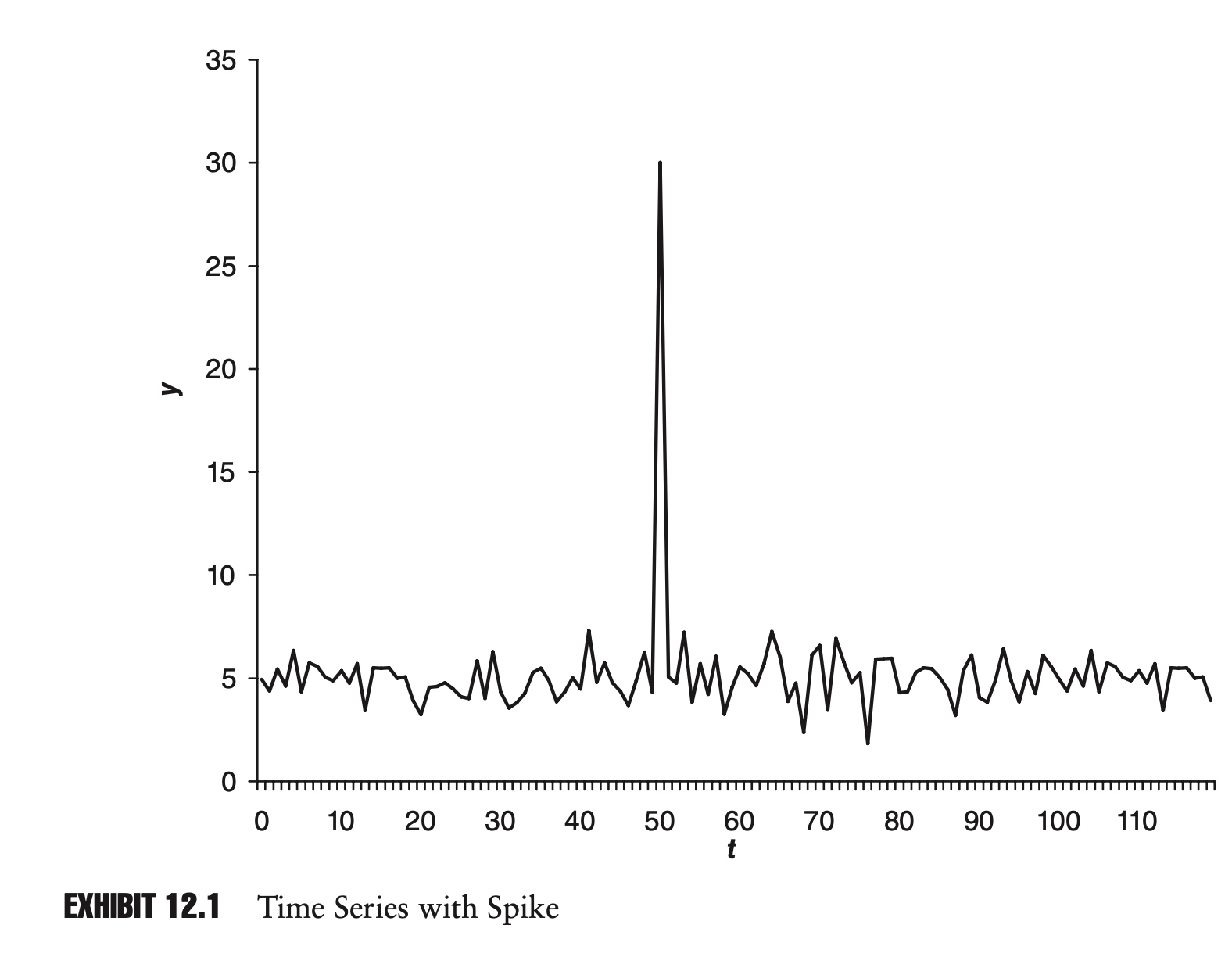
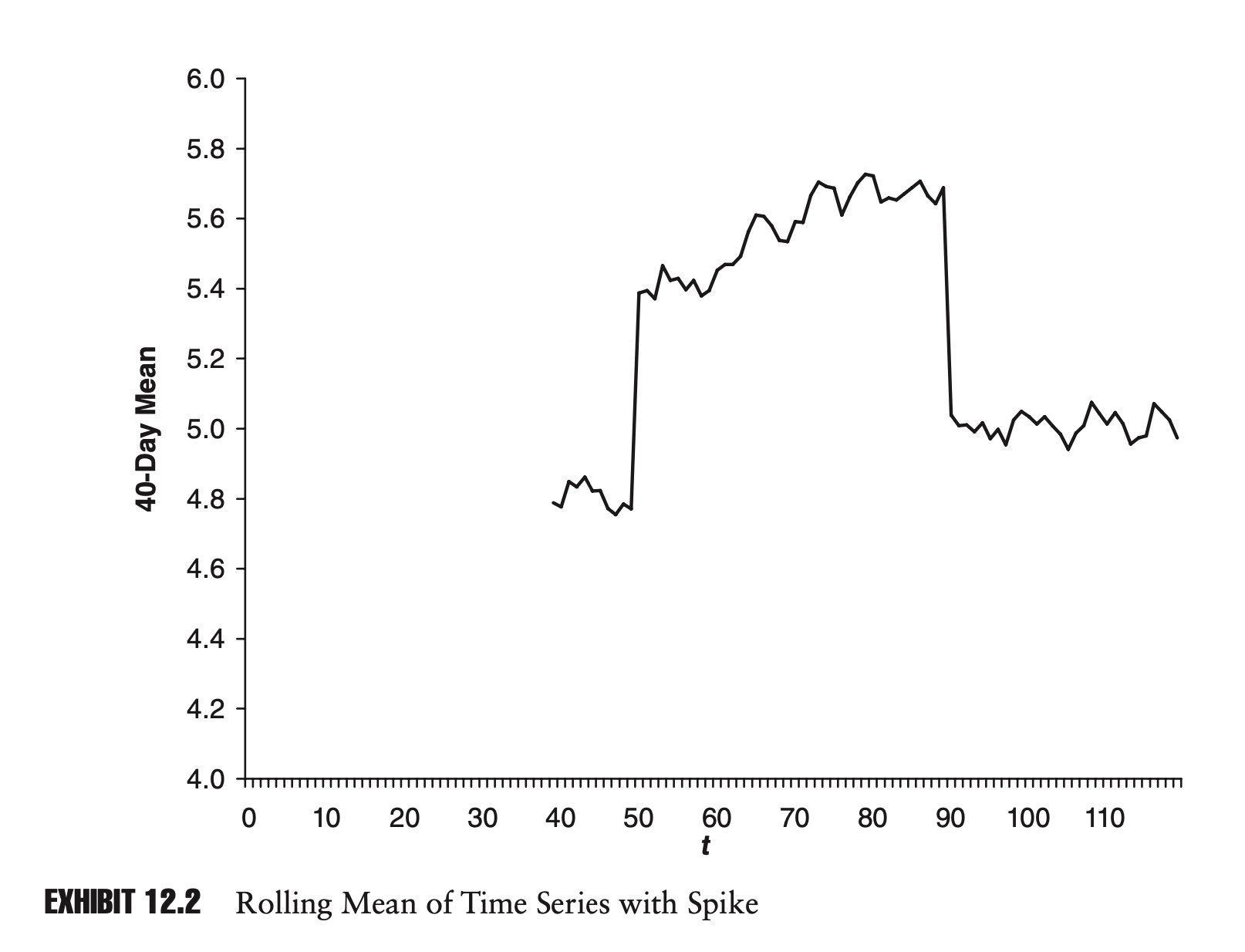
The second objection is more aesthetic. As extreme points enter and leave our data set, this can cause dramatic changes in our estimator. Exhibit 12.1 shows a sample time series. Notice the outlier in the series at time t = 50. Exhibit 12.2 shows the rolling 40-day mean for the series.
Notice how the spike in the original time series causes a sudden rise and drop in our estimate of the mean in Exhibit 12.2. Because of its appearance, this phenomenon is often referred to as plateauing. Technically, there is nothing wrong with plateauing, but many practitioners find this type of behavior unappealing.
In the end, the window length chosen is often arbitrary. While they are convenient and widely used, it is difficult to see why these common window lengths are better than, say, one year plus five days or 142 days.
One approach that addresses many of these objections is known as an exponentially weighted moving average (EWMA). An EWMA is a weighted mean in which the weights decrease exponentially as we go back in time. The EWMA estimator of the mean can be formulated as:
\[\hat{\mu}_{t}=\frac{1-\delta}{1-\delta^{n}} \sum_{i=0}^{n-1} \delta^{i} x_{t-i}\]Here, $\delta$ is a decay factor, where $0 < \delta < 1$. For the remainder of this chapter, unless noted otherwise, assume that any decay factor, $\delta$, is between zero and one. The term in front of the summation is the—by now familiar—inverse of the summation of δ from 0 to n − 1.
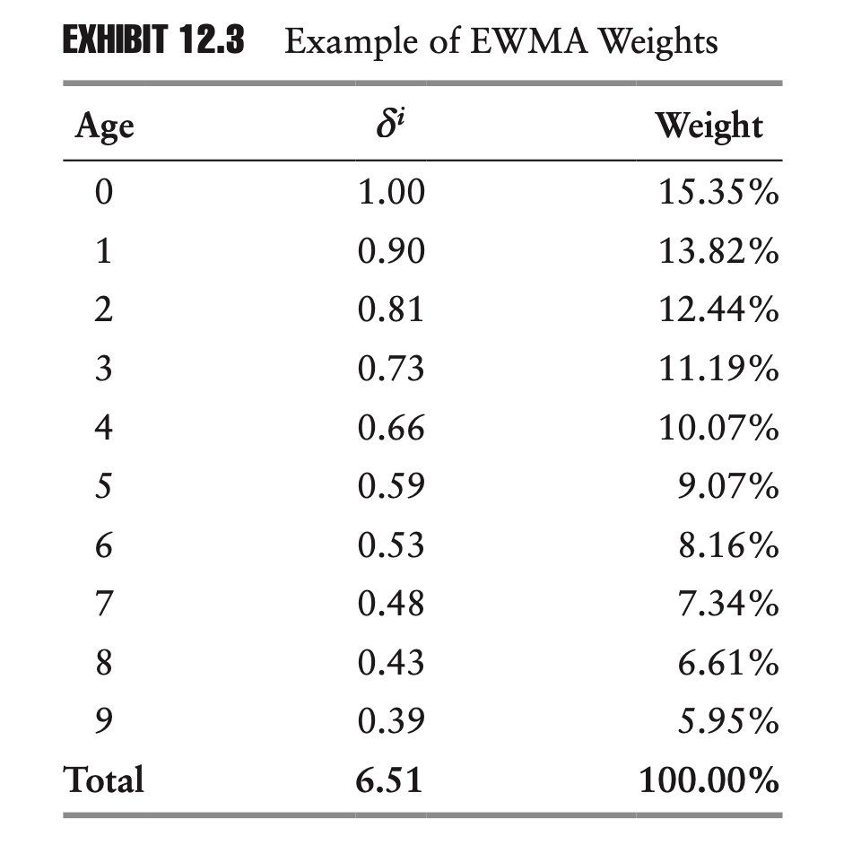
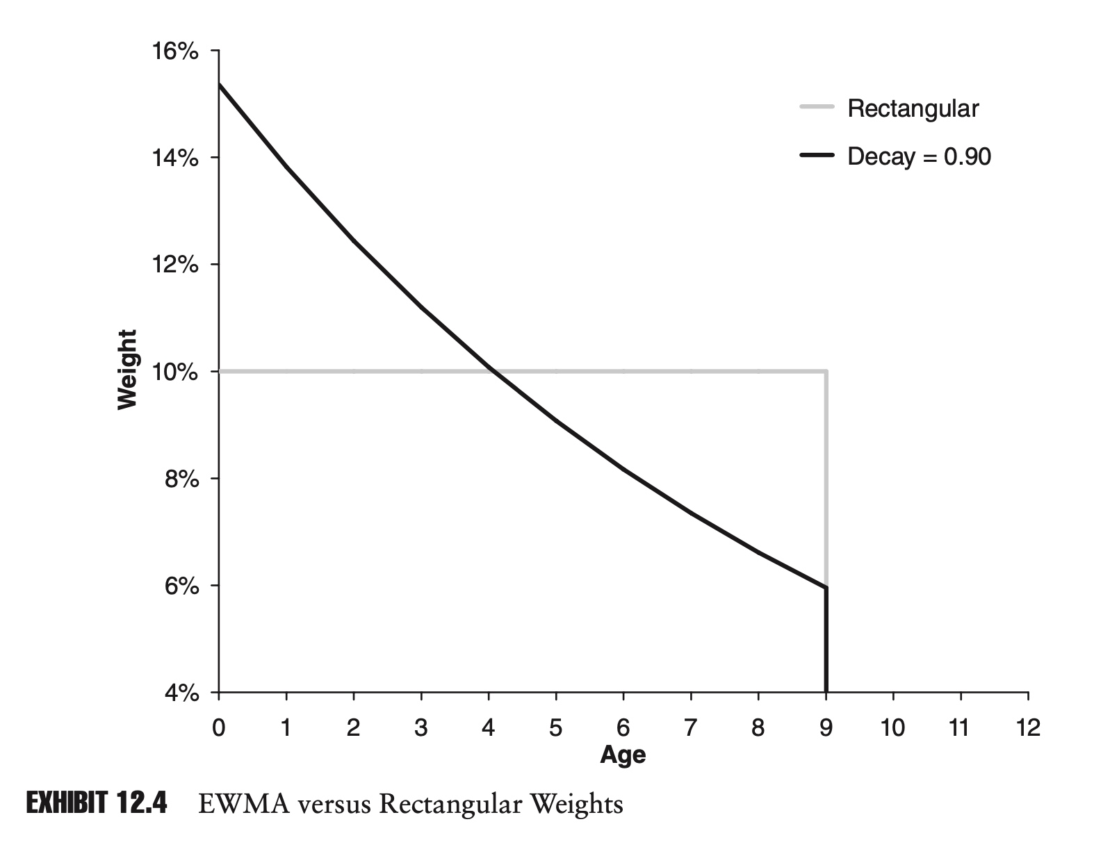
Exhibit 12.4 plots these weights against time, as well as the corresponding weights for the standard equally weighted BLUE.
As you can see, the EWMA weights form a smooth exponential curve that fades at a constant rate as we go back in time. By contrast, because of the shape of the chart, we often refer to the equally weighted estimator as a rectangular window.
One way we can characterize an EWMA is by its half-life. Half of the weight of the average comes before the half-life, and half after. We can find the half-life by solving for h in the following equation:
\[\sum_{i=0}^{h-1}\delta^i=\frac{1}{2}\sum_{i=0}^{n-1}\delta^i\]The solution is:
\[h=\frac{ln(0.5+0.5\delta^n)}{ln(\delta)}\]For a sample of 250 data points and a decay factor of 0.98, the half-life is approximately 34.
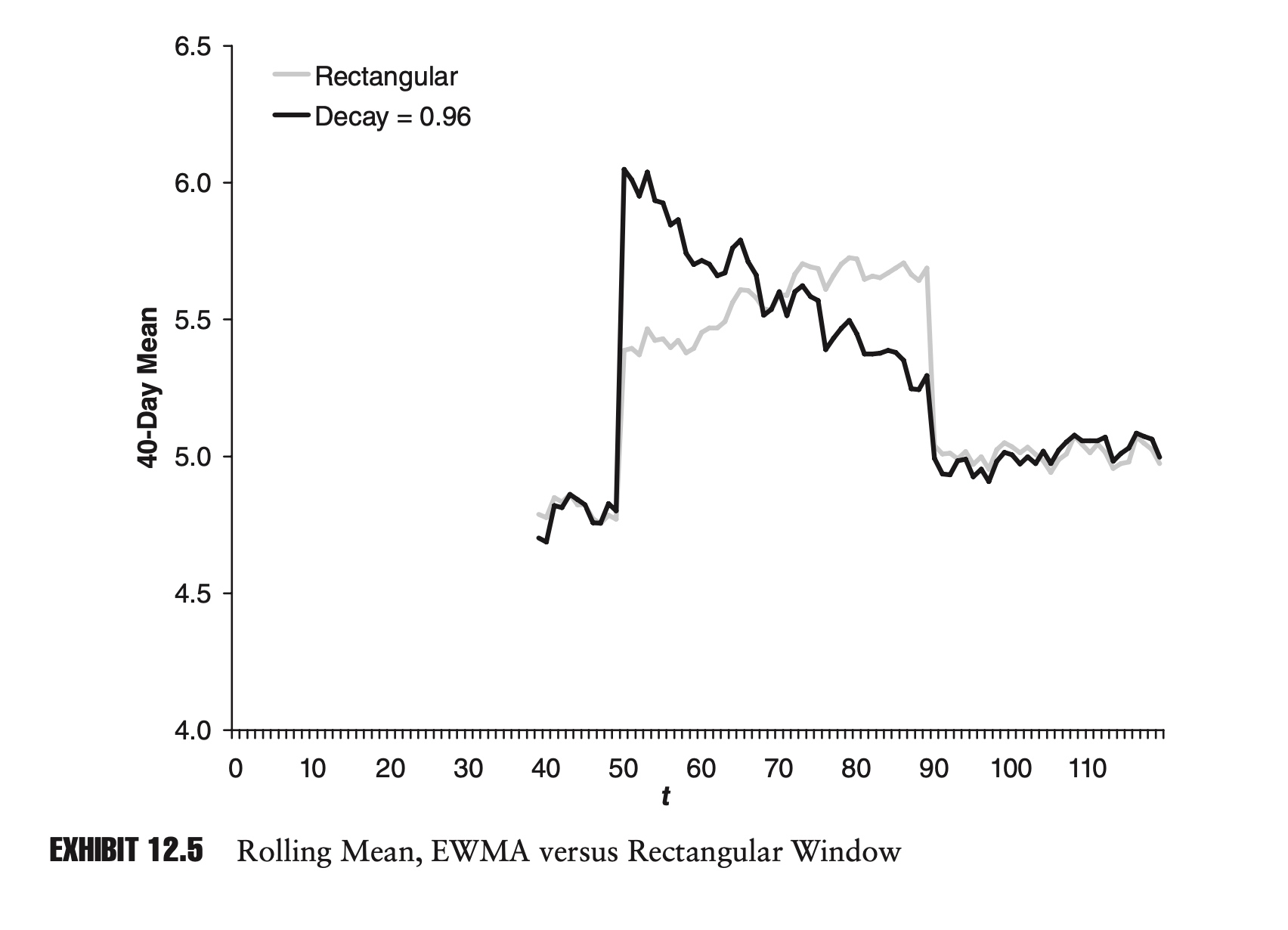
The EWMA can solve the problem of plateauing. The addition of an extreme data point to our data set can still cause a sudden change in our estimator, but the impact of that data point will slowly fade over time.
Besides addressing the aesthetic issue of plateauing, the EWMA estimator also addresses our philosophical objection to fixed windows. Rather than suddenly dropping out of the data set, the weight on any point is slowly reduced over time.
Finally, a fixed window length with a decay factor can be viewed as a compromise between a rectangular window of arbitrary length and using all available data. Because $|\delta|$ is less than one, as n goes to infinity, $\bar{\mu}_t$ can be rewritten as:
\[\bar{\mu}_t=(1-\delta)\sum_{i=0}^{\infty} \delta^i x_{t-i}\]Clearly an infinite series, if it did exist, would be using all available data. In practice, though, for reasonable decay factors, there will be very little weight on points from the distant past. Because of this, we can use a finite window length, but capture almost all of the weight of the infinite series. Using our geometric series math:
\[\frac{\text { Weight of finite series }}{\text { Weight of infinite series }}=\frac{\frac{1-\delta^{n}}{1-\delta}}{\frac{1}{1-\delta}}=1-\delta^{n}\]For a decay factor of 0.98, if our window length is 250, we would capture 99.4% of the weight of the infinite series.
By carefully rearranging the Equation, we can express the EWMA estimator as a weighted average of its previous value and the most recent observation:
\[\hat{\mu}_{t}=(1-\delta) \sum_{i=0}^{\infty} \delta^{i} x_{t-i}=(1-\delta) x_{t}+\delta (1-\delta) \sum_{i=0}^{\infty} \delta^{i} x_{t-i-1}=(1-\delta) x_{t}+\delta \hat{\mu}_{t-1}\]Viewed this way, our EWMA is a formula for updating our beliefs about the mean over time. As new data become available, we slowly refine our estimate of the mean. This updating approach seems very logical, and could be used as a justification for the EWMA approach.
Variance
Just as we used a decay factor when calculating the mean, we can use a decay factor when calculating other estimators. For an estimator of the sample variance, when the mean is known, the following is an unbiased estimator:
\[\hat{\sigma}_{t}^{2}=\frac{1-\delta}{1-\delta^{n}} \sum_{i=0}^{n-1} \delta^{i}\left(r_{t-i}-\mu\right)^{2} \quad 0<\delta<1\]If we imagine an estimator of infinite length, then the term δn goes to zero, and we have:
\[\hat{\sigma}_{t}^{2}=(1-\delta) \sum_{i=0}^{\infty} \delta^{i}\left(r_{t-i}-\mu\right)^{2} \quad 0<\delta<1\]This formula, in turn, leads to a useful updating rule:
\[\hat{\sigma}_{t}^{2}=(1-\delta) \left(r_{t}-\mu\right)^{2}+\delta \hat{\sigma}_{t-1}^{2}\]As with our estimator of the mean, using a decay factor is equivalent to an updating rule. In this case, the new value of our estimator is a weighted average of the previous estimator and the most recent squared deviation.
As mentioned in connection with the standard estimator for variance, it is not uncommon in finance for the mean to be close to zero and much smaller than the standard deviation of returns. If we assume the mean is zero, then our updating rule simplifies even further to:
\[\hat{\sigma}_{t}^{2}=(1-\delta) r_{t}^{2}+\delta \hat{\sigma}_{t-1}^{2}\]In the case where the mean is unknown and must also be estimated, our estimator takes on a slightly more complicated form:
\[\hat{\sigma}_{t}^{2}=A\sum_{i=0}^{n-1}\delta^i r^2_{t-i} -B\bar{\mu}_t^2\]where $\bar{\mu}_t$ is the sample mean, based on the same decay factor, $\delta$, and A and B are constants defined as:
\[\begin{aligned} A &=\frac{S_{1}}{S_{1}^{2}-S_{2}} \\ B &=S_{1} A \\ S_{1} &=\frac{1-\delta^{n}}{1-\delta} \\ S_{2} &=\frac{1-\delta^{2 n}}{1-\delta^{2}} \end{aligned}\]It is not too difficult to prove that in the limit, as $\delta$ approaches one—that is, as our estimator becomes a rectangular window—A approaches 1/(n − 1) and B converges to n/(n − 1). Just as we would expect, in the limit our new estimator converges to the standard variance estimator.
Weighted Least Squares
To apply the same decay factor logic to linear regression analysis, we simply need to multiply all of the sample data, both the regressors and regressands, by the appropriate decay factors. Recall that, for a multivariate regression, the ordinary least squares (OLS) estimator is defined as:
\[\bar{\beta}=(X'X)^{-1}X'Y\]To integrate our decay factor into this analysis, we start by defining $\lambda$ as the square root of our decay factor, $\delta$. Next, we construct a diagonal weight matrix, W, whose diagonal elements are a geometric progression of $\lambda$:
\[\mathbf{W}=\left[\begin{array}{cccc}\lambda^{n-1} & \cdots & 0 & 0 \\ \vdots & \ddots & 0 & 0 \\ 0 & 0 & \lambda & 0 \\ 0 & 0 & 0 & 1\end{array}\right]\]We can then form a new estimator for our regression parameters:
\[\bar{\beta}=(X'W'WX)^{-1}X'W'WY\]This estimator is known as the weighted least squares estimator.
One way to view what we are doing is to redefine our regressors and regressands as follows:
\[\begin{aligned} X^\star&=WX\\ Y^\star&=WY \end{aligned}\]The new matrices take our original data, and multiply the data at time t − i by $\lambda^i$. The effect is to make data points from the distant past smaller, which decreases their variance and decreases their impact on our parameter estimates. With these new matrices in hand, our weighted least squares estimator can now be written as:
\[\bar{\beta}=({X^{\star}}'X^\star)^{-1}{X^{\star}}'Y^\star\]In this way, our weighted least squares estimator can be viewed as the OLS estimator of our transformed data.
One potential problem with the weighted least squares approach, as described here, involves heteroscedasticity. If the initial data set is homoscedastic, then clearly the transformed data will be heteroscedastic. As with our mean and variance estima- tors, when we use a decay factor, the resulting estimator will be unbiased, but it will not be the BLUE.
CrashMetrics approach
In theory, there is an infinite number of possible weighting schemes we could use, but one novel approach pioneered by Philip Hua and Paul Wilmott is worth mentioning (Hua and Wilmott 1997).
As risk managers, if we are ultimately concerned with extreme markets, then the suggestion is that we should be placing more weight on data from extreme markets, and little or no weight on data from normal markets. This approach seems particularly appropriate for stress testing, where, by definition, we are dealing with extreme events.
One way to implement this approach would be to define a cutoff return that separates extreme markets and normal markets, and use only the data from extreme markets to calculate statistics (weights are zero or one). Alternatively, we could define weights as a function of how extreme the returns are (e.g., the weights are equal to the square of the return of a given index). When applied to stress testing or value at risk (VaR), Hua and Wilmott refer to this as the CrashMetrics approach. Looked at more generally, it provides a novel third way of calculating sample parameters.
Application: Hybrid VaR
One of the simplest approaches to estimating value at risk (VaR) is the historical method or historical simulation. In this approach, we calculate the backcast returns of a portfolio of assets, and take these as the portfolio’s return distribution. To calculate the 95th percentile VaR, we would simply find the least worst of the worst 5% of returns. For example, suppose we have 100 returns, ranked from lowest to highest:
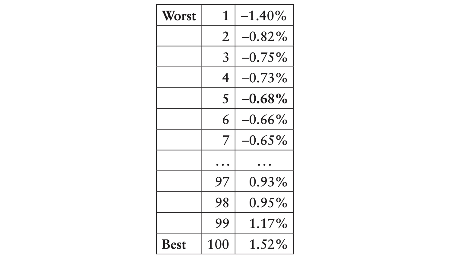
Here the 95th percentile VaR would correspond to the fifth return, −0.68%.
Instead of giving equal weight to all data, we can use a decay factor to weight more recent data more heavily. Rather than finding the fifth worst return, we would order the returns and find the point where we have 5% of the total weight:

In this case, we get to 5% of the total weight between the third and fourth returns. At this point there are two approaches. The more conservative approach is to take the third return, −0.75%. The alternative is to interpolate between the third and fourth returns, to come up with −0.74%.
This general approach, using historical returns with decreasing weights, is often called the hybrid approach because it combines aspects of standard historical simulation and weighted parametric approaches; see, for example, Allen, Boudoukh, and Saunders (2004).
Comments