Asset Pricing Methods

Overview

For asset pricing, we have the following approaches:

• Replication
• Adjusting for risk premium (Market Price for Risk)
• Risk-neutral Pricing
  • Discrete: Tree model
  • Continuous: Martingale approach
• PDE approach

In fact, these are equivalent ways of pricing. There is no “best” method, and we should choose a method depending on the context.

Framework

Binomial Model Framework

For simplicity, let’s assume a binomial model framework, which can be easily extended to multi-steps or continuous models (e.g. Black-Scholes models). It is also extensively used by practitioners to price real securities.

The binomial model: We assume that we have a risk-free asset $D_t$, and a risky asset $S_t$. For simplicity, we call $S_t$ as stock price.

A short tick later(Δt),the stock price can jump up to $S_u$ with probability p and jump down to $S_d$ with probability (1-p).

The bond price is not random. Let r be the continuously compounded risk-free rate. If the initial price of a cash bond is $D_0 =1$, then a short tick later, the bond price will grow to $D_0*e^{r\Delta t}=e^{r\Delta t}$

A derivative paysoff $f_u$ if the stock price goes up and $f_d$ if the stock price goes down.

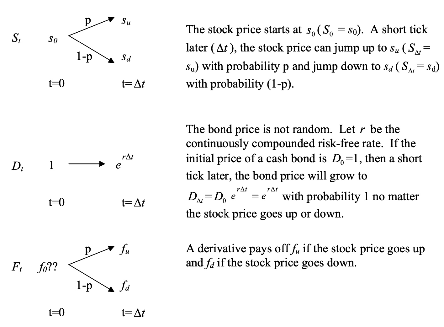
Question: What is the initial price of the derivative?

The unconscious statistician might pay \(f =e^{−rΔt} (pf_u +(1−p)f_d )\) ,i.e.the expectation of future payoffs discounted by the risk-free rate.

But, this answer is wrong. Since there is uncertainty in the future price of $f$, investors require risk-premium to take the risk. Therefore, we need to add risk-premium to the discounted rate.

Market price of risk. The market price of risk is compensation per unit of risk. In the binomial model: $$\lambda_{0}=\frac{\text { risk premium }}{\text { amount of risk }}=\frac{e^{-r_{0} \Delta} \mathbb{E}_{0}\left[P_{1}\right]-P_{0}}{P_{1, u}-P_{1, d}}$$ where $$\mathbb{E}_{0}\left[P_{1}\right]=p_{u} P_{1, u}+p_{d} P_{1, d}$$

Equivalent definition in terms of returns:

\[P_{0}=e^{-r_{0} \Delta} \mathbb{E}_{0}\left[P_{1}\right]-\lambda_{0}\left(P_{1, u}-P_{1, d}\right)\]

So far, we have no idea how to “price” this MPR term.

Black-Scholes Framework

In the original Black-Scholes economy:
1. There are no market imperfections. That is, there are no taxes, no transactions costs, and no short-sale constraints. Security trading is frictionless;
2. security trading is continuous;
3. there is unlimited risk-free borrowing and lending at the constant continuously compounded risk-free rate r .
4. the stock price follows a geometric Brownian motion with constant growth rate μ and constant volatility parameter σ $$dSt =\mu S_t dt+\sigma S_t dBt,$$ where $B_t$ is a standard Brownian motion under P-measure;
5. there are no dividends during the life of the derivative to be evaluated;
6. there are no risk-less arbitrage opportunities.

Ito’s lemma: a formula used to calculate explicitly the stochastic differential equation (SDE) that governs the dynamics of an arbitrary function given the stochastic process of the function’s arguments.

Let x follows the SDE $$dx = μ_1 dt +\sigma_1 dB_t^x$$, then the SDE of $f (x,t)$ given the stochastic process of x is: $$d f(x, t)=\frac{\partial f}{\partial t} d t+\frac{\partial f}{\partial x} d x+\frac{1}{2} \frac{\partial^{2} f}{\partial x^{2}}(d x)^{2}$$
Let x and y follows the SDEs $$dx = μ_1 dt +\sigma_1 dB_t^x$$ and $$dy = μ_2 dt +\sigma_2 dB_t^y$$, with $$dB_t^x *dB_t^y =\rho dt$$, then the SDE of $f (x, y,t)$ given the stochastic process of x and y is: $$\begin{aligned} d f(x, y, t)=& \frac{\partial f}{\partial t} d t+\frac{\partial f}{\partial x} d x+\frac{\partial f}{\partial y} d y \\ &+\frac{1}{2}\left[\frac{\partial^{2} f}{\partial x^{2}}(d x)^{2}+\frac{\partial^{2} f}{\partial y^{2}}(d y)^{2}+2 \frac{\partial^{2} f}{\partial x y}(d x d y)\right] \end{aligned}$$

Ito’s lemma basically says that we need to do Taylor’s expansion to the second order. The multiplication rules for stochastic differentials:

\[\begin{array}{c|ccc} \mathrm{x} & d B^{x} & d B^{y} & d t \\ \hline d B^{x} & d t & \rho d t & 0 \\ d B^{y} & & d t & 0 \\ d t & & & 0 \end{array}\]

Modeling of the Stock Price

We typically model stock prices as a geometric Brownian motion or lognormal diffusion under measure P:

\[dS_t=\mu dS_t + \sigma S_t dB_t\]

with a constant growth rate $\mu$ and a constant diffusion parameter $\sigma$.

If the underlying stock does not distribute dividends, then $\frac{dS_t}{S_t}$=The return of investment over the period of [t,t+dt] is given by:

\[\text{expected return } μ dt + \text{unexpected return } σ dBt.\]

In a risk-neutral world: \(dS_t=r S_t dt + \sigma S_t dB^Q_t\)

The following two proposition is equivalent:
1. The log-price $p_t=lnS_t$ follows a Brownian motion $$d p_{t}=\left(\mu-\frac{1}{2} \sigma^{2}\right) d t+\sigma d B_{t}$$ 2. $S_t$ follows a geometric Brownian motion $$dS_t=\mu S_t dt+ \sigma S_t dB_t$$

It is easy to prove with Ito’s lemma. In fact:

\[\begin{aligned} d p_{t} &=\frac{\partial p_{t}}{\partial t} d t+\frac{\partial p_{t}}{\partial S_{t}} d S_{t}+\frac{1}{2} \frac{\partial^{2} p_{t}}{\partial S_{t}^{2}}\left(d S_{t}\right)^{2} \\ &=\frac{1}{S_{t}}\left(\mu S_{t} d t+\sigma S_{t} d B_{t}\right)+\frac{1}{2}\left(-\frac{1}{S_{t}^{2}}\right)\left(\mu S_{t} d t+\sigma S_{t} d B_{t}\right)^{2} \\ &=\left(\mu-\frac{1}{2} \sigma^{2}\right) d t+\sigma d B_{t} \end{aligned}\]

Similarly,we can show that p follows \(dp_t=\left(r-\frac{1}{2} \sigma^{2}\right) d t+\sigma d B^Q_{t}\) under the risk-neutral measure Q

The log-price $p_t=lnS_t$ follows a geometric Brownian

A random variable Y is log-normally distributed if the natural logarithm of it, X, is a normal random variable. $$X\sim N(\mu,\sigma)$$ $$Y=e^{X}\sim LN(\mu,\sigma)$$

• The probability density function of a lognormal random variable is:

\[f(y)=\frac{1}{\sqrt{2 \pi} \sigma y} e^{-\frac{(\ln y-\mu)^{2}}{2 \sigma^{2}}}, 0 \leq y<+\infty\]

• The mean and the variance of a lognormal random variance are

\[E(Y)=e^{\mu+\frac{1}{2}\sigma^2}\] \[V(Y)=e^{2\mu+\sigma^2}(e^{\sigma^2}-1)\]

Application

Since $dlnS_t=dp_t=\left(r-\frac{1}{2} \sigma^{2}\right) d t+\sigma d B^Q_{t}$, we have

\[lnS_T=lnS_0 +\left(r-\frac{1}{2} \sigma^{2}\right) T+\sigma (B_T-B_0)\]

Therefore, log price at maturity \(lnS_T \sim N(\mu_*,\sigma_*^2)\)

where \(\mu=lnS_0 +\left(r-\frac{1}{2} \sigma^{2}\right) T\) and \(\sigma_*^2=\sigma^2 T\).

Therefore, the density function of $S_T$ is

\[f(S(T))=\frac{1}{\sqrt{2 \pi} \sigma \sqrt{T} S(T)} e^{-\frac{\left(\ln \frac{S(T)}{S(0)}\left(r-\frac{1}{2} \sigma^{2}\right) T\right)^{2}}{2 \sigma^{2} T}}\] \[E(S_T)=e^{\mu_* + \frac{1}{2}\sigma_*^2}=S(0)e^{rT}\]

Replication

First let’s introduce some important concepts:

The simultaneous buying and selling of a security at two different prices in two different markets, resulting in profits without risk. Perfectly efficient markets present no arbitrage opportunities. Perfectly efficient markets seldom exist, but, arbitrage opportunities are often precluded because of transactions costs.

There is no arbitrage opportunity in financial markets.

Based on this principle, we have the following law:

If two securities have the same payoffs in the future, then they must have the same price today.

A replicating portfolio of a security with payoffs $P_u$ and $P_d$ in the two node $u$ and $d$ at time 1 is a portfolio of $D$ and $S$ that exactly replicates the values of the security at time 1.

We construct a portfolio out of the stock and the cash bond to mimic the payoffs of the derivative. This portfolio is called “replicating portfolio.” Then the price of the derivative must be the same as the price of the replicating portfolio by the law of one price.

Let x be the stock holding strategy and let y be the bond holding strategy. The unit of x and y is number of shares. Then the price and the payoffs of the portfolio are as shown in the following diagram:

\[\left\{\begin{array}{l} x s_{u}+y e^{r \Delta t}=f_{u} \\ x s_{d}+y e^{r \Delta t}=f_{d} \end{array}\right.\]

By the law of one price, this must also be the price of the derivative otherwise there exists an arbitrage opportunity.

\[f_{0}=x s_{0}+y=e^{-r \Delta t}\left(\frac{e^{r \Delta t} s_{0}-s_{d}}{s_{u}-s_{d}} f_{u}+\left(1-\frac{e^{r \Delta t} s_{0}-s_{d}}{s_{u}-s_{d}}\right) f_{d}\right)\]

The above procedure implies several points:

• To construct a replicating portfolio, we should buy $x=\frac{f_{u}-f_{d}}{s_{u}-s_{d}}$ shares of the stock
• For any risky-asset, we can always form $x,y$, s.t. $xS_0+yD_0$ will replicate the payoffs of the risky-asset

Risk-neutral pricing

In last part, we show:

\[f_{0}=x s_{0}+y=e^{-r \Delta t}\left(\frac{e^{r \Delta t} s_{0}-s_{d}}{s_{u}-s_{d}} f_{u}+\left(1-\frac{e^{r \Delta t} s_{0}-s_{d}}{s_{u}-s_{d}}\right) f_{d}\right)\]

Let $q=\frac{e^{r \Delta t} s_{0}-s_{d}}{s_{u}-s_{d}}$, then

\[f_{0}=x s_{0}+y=e^{-r \Delta t}\left(qf_u+ (1-q)f_d\right)\]

This Pricing formula looks like what we want — the price of the derivative is the expectation of the future payoffs discounted at the risk-free rate!

The following are equivalent:
1. There is No Arbitrage
2. There exist valid risk-neutral probabilities
(That is, $q\in [0,1]$ in the case of the one-step binomial model.)

For $q=\frac{e^{r \Delta t} s_{0}-s_{d}}{s_{u}-s_{d}}$, we can prove that $q\in [0,1]$ by non-arbitrage assumption.

For example, $e^{r\Delta t}s_0 \geq s_d$, otherwise there is an arbitrage opportunity by short D and long S.

So, q is the “risk-neutral probability.” A collection of risk-neutral probabilities ${ q , 1 − q }$ on the set of all possible outcomes {up, down} is called risk-neutral probability measure or simply risk-neutral measure, denoted by $\mathcal{Q}$.

The price of the derivative is the expected future payoffs under the risk-neutral measure Q discounted by the risk-free rate.

\[f_{0}=x s_{0}+y=e^{-r \Delta t}\left(qf_u+ (1-q)f_d\right)\]

Note, q depends only on the risk-free rate r, current stock price $s_0$ and the future possible stock prices $s_u$ and $s_d$. It does not depend on the true probability p at all.

Summary: 5-step risk-neutral derivative pricing rule in the binomial branch framework

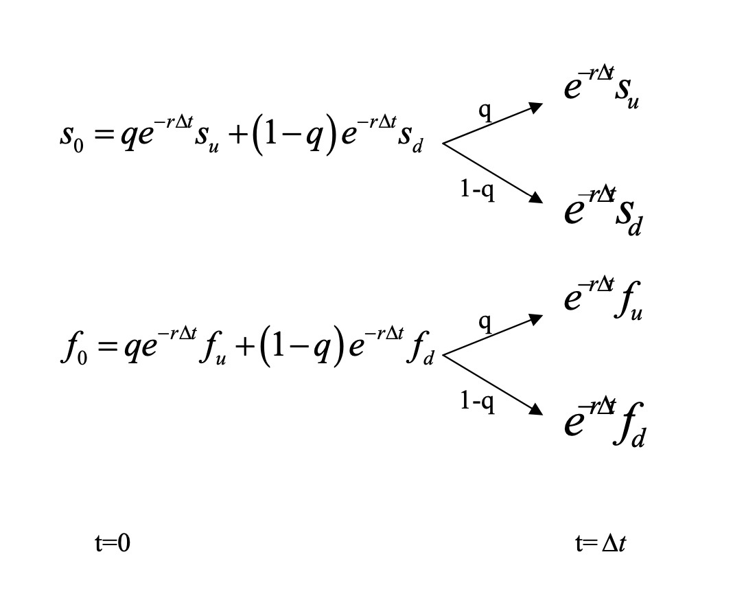
• Step 1: Discount the stock price, $S_{Δt}$ , by using risk-free rate to have discounted stock price, $e^{−rΔt} S_{Δt}$ ;
• Step 2: Find a measure Q that makes the discounted stock price a martingale;
• Step 3: Discount the derivative, $f_{Δt}$ , by using risk-free rate to have discounted stock price, $e^{−rΔt} f_{Δt}$ ;
• Step 4: Calculate the expectation of the discounted derivative price under measure Q.
• Step 5: Calculate hedge ratio $x=\frac{f_u-f_d}{s_u-s_d}$, s.t. $f=xS+yD$

Martingale Approach

A process $X_t$ is a martingale with respect to a measure Ρ if it satisfies the following two conditions：
(i) $E^{P}\left(X_{T} \mid X_{t}, \ldots, X_{0}\right)=X_{t},$ for all $T>t,$ and
(ii) $E^{P}\left(\left|X_{T}\right|\right)<\infty,$ for all $T$

A martingale measure of a process is the measure that makes the process a martingale.

Therefore, the risk-free discounted stock price is a martingale under the risk-neutral measure Q.

Since any risky asset can be expressed as $f=x_tS_t +y_tD_t$, he risk-free discounted derivative is also a martingale under the risk-neutral measure Q. So the risk-neutral measure Q is also called “equivalent martingale measure.”

The 5-step risk-neutral pricing rule works in the continuous-time. The difference from the discrete-time is that we now have to identify the density function of the underlying under the risk-neutral probability measure and then do an integration to evaluate the risk-neutral expectation of the discounted derivative payoff.

Specifically, we have the Harrison-Pliska (1981) risk-neutral valuation formula.

\[\begin{array}{c} c\left(S_{0}, 0\right)=e^{-r T} E^{Q}\left(c\left(S_{T}, T\right)\right) \\ c\left(S_{t}, t\right)=e^{-r(T-t)} E_{t}^{Q}\left(c\left(S_{T}, T\right)\right) \end{array}\]

Market Price of Risk

The market price of risk is compensation per unit of risk. In the binomial model: $$\lambda_{0}=\frac{\text { risk premium }}{\text { amount of risk }}=\frac{e^{-r_{0} \Delta} \mathbb{E}_{0}\left[P_{1}\right]-P_{0}}{P_{1, u}-P_{1, d}}$$ where $$\mathbb{E}_{0}\left[P_{1}\right]=p_{u} P_{1, u}+p_{d} P_{1, d}$$

Equivalent definition in terms of returns:

\[P_{0}=e^{-r_{0} \Delta} \mathbb{E}_{0}\left[P_{1}\right]-\lambda_{0}\left(P_{1, u}-P_{1, d}\right)\]

So far, we have no idea how to “price” this MPR term.

We can easily prove that all risky asset has a same MPR $\lambda$, by the replication approach $f=xS+yD$.

Risk-neutral vs. physical probabilities

Physical probabilities ($p_u$ and $p_d$ in the context of the binomial model) describe the actual likelihood of events occurring.

Risk-neutral probabilities ($q_u$ and $q_d$ in the context of the binomial model) follow from No Arbitrage and is a construct used for pricing.

What is the relationship between the two? How do we interpret this relationship?

Consider an asset which only pays 1 in state $u$ and zero otherwise.

We can price asset using the MPR approach:

\[P_0=p_u e^{-r_0 \Delta}-\lambda_0(1-0)\]

We can also use risk-neutral pricing:

\[P_0=q_ue^{-r_0 \Delta}\]

Since the two are equal:

\[p_u^*:=q_u=p_u-\lambda_0 e^{r_0\Delta}\]

Similarly,

\[p_d^*:=q_d=p_d +\lambda_0 e^{r_0\Delta}\]

Summary:

\[\begin{array}{l} p_{u}^{*}=p_{u}-\lambda_{0} e^{r_{0} \Delta} \\ p_{d}^{*}=p_{d}+\lambda_{0} e^{r_{0} \Delta} \end{array}\]

For $\lambda_0=0$, they are the same.

PDE approach

The Black-scholes formula for the price of vanilla call/put options is a function of five arguments.

Let $c_t$ be the price of a option at time t; Let $S_t$ be the underlying stock price at time t; Let $τ = T − t$ be the time-to-maturity, where T is the maturity time; Let K be the strike price; Let r be the constant risk-free rate; Let σ be the return volatility of the underlying stock; Then $c_t =C(S_t,\tau=T−t;K,r,σ)$. The option price $c_t$ is the dependent variable. The current stock price $S_t$ and the current time t are the independent variables. The rest are parameters.

Assume the stock price St follows a geometric Brownian motion:

\[dS_t=\mu S_t dt+ \sigma S_tdB_t\]

By Ito’s lemma, we can derive the differential expression of the option price:

\[\begin{aligned} d c_{t} &=\frac{\partial c_{t}}{\partial t} d t_{t}+\frac{\partial c_{t}}{\partial S_{t}} d S_{t}+\frac{1}{2} \frac{\partial^{2} c_{t}}{\partial S_{t}^{2}}\left(d S_{t}\right)^{2} \\ &=\frac{\partial c_{t}}{\partial t} d t_{t}+\frac{\partial c_{t}}{\partial S_{t}}\left(\mu S_{t} d t+\sigma S_{t} d B_{t}\right)+\frac{1}{2} \frac{\partial^{2} c_{t}}{\partial S_{t}^{2}} \sigma^{2} S_{t}^{2} d t \\ &=\left(\frac{\partial c_{t}}{\partial t}+\frac{1}{2} \frac{\partial^{2} c_{t}}{\partial S_{t}^{2}} \sigma^{2} S_{t}^{2}+\mu S_{t} \frac{\partial c_{t}}{\partial S_{t}}\right) d t+\sigma S_{t} \frac{\partial c_{t}}{\partial S_{t}} d B_{t} \end{aligned}\]

Let us long one unit of the option and short Δ units of the stock. The price of the portfolio at time t is:

\[P_t=c_t-\Delta S_t\]

The instantaneous dollar return on the portfolio is:

\[\begin{aligned} d P_{t} &=d c_{t}-\Delta d S_{t} \\ &=\left(\frac{\partial c_{t}}{\partial t}+\frac{1}{2} \frac{\partial^{2} c_{t}}{\partial S_{t}^{2}} \sigma^{2} S_{t}^{2}+\mu S_{t}\left(\frac{\partial c_{t}}{\partial S_{t}}-\Delta\right)\right) d t+\sigma S_{t}\left(\frac{\partial c_{t}}{\partial S_{t}}-\Delta\right) d B_{t} \end{aligned}\]

By choosing $\Delta=\frac{\partial C_t}{\partial S_t}$, we ge want a risk-neutral portfolio. Such a portfolio is said to be perfectly hedged or Delta-neutral portfolio

Since P becomes risk-free asset, now we have: \(dP_t=rP_tdt\)

After regrouping, we have the well-known Black and Scholes partial differential equation (PDE):

\[\frac{\partial c_{t}}{\partial t}+\frac{1}{2} \sigma^{2} S_{t}^{2} \frac{\partial^{2} c_{t}}{\partial S_{t}^{2}}+r S_{t} \frac{\partial c_{t}}{\partial S_{t}}-r c_{t}=0\]

This PDE is a second-order linear parabolic PDE for the option price $c_t$ subject to the following boundary condition:

\[C_T(S_T,T)=Max(S_T-K,0)\]

The unique solution to this PDE is the famous Black-Scholes formula:

\[\begin{array}{l} c\left(S_{t}, t\right)=S_{t} \Phi\left(d_{1}\right)-K e^{-r(T-t)} \Phi\left(d_{2}\right) \\ d_{1}=\frac{\ln \left(\frac{S_{t}}{K}\right)+\left(r+\frac{1}{2} \sigma^{2}\right)(T-t)}{\sigma \sqrt{T-t}} \\ d_{2}=\frac{\ln \left(\frac{S_{t}}{K}\right)+\left(r-\frac{1}{2} \sigma^{2}\right)(T-t)}{\sigma \sqrt{T-t}} \end{array}\]

where $\Phi(\cdot)$ is the standard normal cumulative distribution function.

How to solve the PDE for different Derivatives?

Heat equation: The temperature in a metal rod satisfies the standard heat equation with an initial condition $f (x_0,0)$

\[\left\{\begin{array}{l} \frac{\partial f}{\partial t}-\frac{1}{2} \sigma^{2} \frac{\partial^{2} f}{\partial x^{2}}=0 \\ f\left(x_{0}, 0\right) \end{array}\right.\]

Delta function $\delta ( x − x_0 )$ is defined as:

\[\delta\left(x-x_{0}\right)=\left\{\begin{array}{l} 0 \quad x \neq x_{0} \\ +\infty \quad x=x_{0} \end{array}\right. \text { and } \int_{-\infty}^{\infty} \delta\left(x-x_{0}\right) d x=1\]

Green’s function $G(x,t; x0 )$ : Green’s function is a solution of the standard heat equation with a particular initial condition, which is the delta function $\delta ( x − x_0 )$ :

\[\left\{\begin{array}{l} \frac{\partial G}{\partial t}-\frac{1}{2} \sigma^{2} \frac{\partial^{2} G}{\partial x^{2}}=0 \\ G\left(x, 0 ; x_{0}\right)=\delta\left(x-x_{0}\right) \end{array}\right.\]

The formula for Green’s function, which is the solution of the above PDE system, is

\[G\left(x, t ; x_{0}\right)=\frac{1}{\sqrt{2 \pi} \sigma \sqrt{t}} e^{-\frac{\left(x-x_{0}\right)^{2}}{2 \sigma^{2} t}}\]

As shown, Green’s function is like a density function of a normal random variable x with mean $x_0$ and variance $σ^2t$ conditional on the initial state x .

The solution of the standard heat equation with an arbitrary initial condition $f (x_0,0)$ can be written in terms of Green’s function as

\[f(x, t)=\int_{-\infty}^{+\infty} f\left(x_{0}, 0\right) G\left(x, t ; x_{0}\right) d x_{0}\]

Summary of PDE approach:

Step 1: Transformation.

Let

\[\begin{array}{l} \tau=T-t \\ c(S, t)=e^{-r \tau} K f(x, \tau) \\ S=K e^{-\left(r-\frac{1}{2} \sigma^{2}\right) \tau+x} \\ x=\ln \frac{S}{K}+\left(r-\frac{1}{2} \sigma^{2}\right) \tau \end{array}\]

TheBlack-Scholes PDE:

\[\frac{\partial c_{t}}{\partial t}+\frac{1}{2} \sigma^{2} S_{t}^{2} \frac{\partial^{2} c_{t}}{\partial S_{t}^{2}}+r S_{t} \frac{\partial c_{t}}{\partial S_{t}}-r c_{t}=0\]

becomes:

\[\left\{\begin{array}{l} \frac{\partial f}{\partial \tau}-\frac{1}{2} \sigma^{2} \frac{\partial^{2} f}{\partial x^{2}}=0 \\ f\left(x_{0}, 0\right) \end{array}\right.\]

The given boundary condition $c(S_T ,T)$ becomes:

\[f(x_0,0)=\frac{e^{r*0}}{K}*c(S_T ,T)\]

Example for vanilla European call, the new PDE system after transformation is

\[\left\{\begin{array}{l} \frac{\partial f}{\partial \tau}-\frac{1}{2} \sigma^{2} \frac{\partial^{2} f}{\partial x^{2}}=0 \\ f\left(x_{0}, 0\right)=\operatorname{Max}\left(e^{x_{0}}-1,0\right) \end{array}\right.\]

Step 2: Solve the new PDE

The transformed PDE system is a standard heat equation with an arbitrary initial condition. We know the solution to the transformed PDE system is

\[f(x, \tau)=\int_{-\infty}^{+\infty} f\left(x_{0}, 0\right) G\left(x, \tau ; x_{0}\right) d x_{0}\] \[G\left(x, t ; x_{0}\right)=\frac{1}{\sqrt{2 \pi} \sigma \sqrt{t}} e^{-\frac{\left(x-x_{0}\right)^{2}}{2 \sigma^{2} t}}\]