Roadmap for the course
- Part I:
- Introduction to basic fixed income concepts
- Pricing in a model free framework
- Lack of models: limited amount of assets that we can price
- Part II:
- Binomial models of interest rates
- Part III:
- More sophisticated interest rate models
Basic Concepts
In other words, $Z(t,T)$ is the price of ZCB at time t, with maturity at T and Notional Amount of 1.
Yields on Treasury notes and bonds, corporate bonds, and municipal bonds are quoted on a semi-annual bond basis (SABB) because their coupon payments are made semi-annually. Compounding occurs twice per year, using a 365-day year.
See Treasury Yield Curve Methodology
Because of its analytical convenience, in this text we mostly use the continuously compounded interest rate in the description of discount factors, and for other quantities.
Translating such a number into another compounding frequency is immediate from Equation:
\[e^{-r(t, T)(T-t)}=Z(t, T)=\frac{1}{\left(1+\frac{r_{n}(t, T)}{n}\right)^{n \times(T-t)}}\]which, more explicitly, implies
\[\begin{array}{r} r(t, T)=n \times \ln \left(1+\frac{r_{n}(t, T)}{n}\right) \\ r_{n}(t, T)=n \times\left(e^{\frac{r(t, T)}{n}}-1\right) \end{array}\]Quoting Conventions:
Treasury Bills: Treasury bills are quoted on a discount basis. That is, rather than quoting a price $P_{bill}(t,T)$ for a Treasury bill, Treasury dealers quote the following quantity
\[d=\frac{100-P_{\text {bill }}(t, T)}{100} \times \frac{360}{n}\]Given a quote d from a Treasury dealer, we can compute the price of the Treasury bill:
\[P_{\text {bill }}(t, T)=100 \times\left[1-\frac{n}{360} \times d\right]\]Treasury Coupon Notes and Bonds.
Coupon notes and bonds present an additional complication. Between coupon dates, interest accrues on the bond. If a bond is purchased between coupon dates, the buyer is only entitled to the portion of the coupon that accrues between the purchase date and the next coupon date. The seller of the bond is entitled to the portion of the coupon that accrued between the last coupon and the purchase date.
It is market convention to quote Treasury notes and bonds without any inclusion of accrued interests. However, the buyer agrees to pay the seller any accrued interest between the last coupon date and purchase price. That is, we have the formula:
Invoice price = Quoted price + Accrued interest
The quoted price is sometimes referred to as the clean price while the invoice price is sometimes also called dirty price.
The accrued interest is computed using the following intuitive formula:
\[\begin{aligned} \text{Accrued interest}=&\text{Interest due in the full period} \times \\ &\frac{\text{Number of days since last coupon date}}{\text{Number of days between coupon payments}} \end{aligned}\]Market conventions also determine the methodology to count days. There are three main ways:
- Actual/Actual: Simply count the number of calendar days between coupons;
- 30/360: Assume there are 30 days in a month and 360 in a year;
- Actual/360: Each month has the right number of days according to the calendar, but there are only 360 days in a year.
Which convention is used depends on the security considered. For instance, Treasury bills use actual/360 while Treasury notes and bonds use the actual/actual counting convention.
Let $P_Z(t,T)$ denote the price of the Zero-Coupon bond at time t with maturity at T and notional amount of 100.
Let $P_C(t,T)$ denote the price of the semiannual coupon bond at time t with maturity at T and notional amount of 100.
Some rate of returns:
1 - LIBOR forward rate:
\[\begin{array}{c} 1+(T-S) L(t, S, T)=\frac{P(t, S)}{P(t, T)} \\ L(t, S, T)=\frac{P(t, S)-P(t, T)}{(T-S) P(t, T)} \end{array}\]2 - LIBOR spot rate:
\[L(S, T)=L(S, \mathrm{~S}, T)=\frac{1-P(S, T)}{(T-S) P(S, T)}\]3 - Continuously compounded forward rate:
\[\begin{array}{c} 1 \times e^{R(T-S)}=\frac{P(t, S)}{P(t, T)} \\ R(t, S, T)=\frac{\log P(t, S)-\log P(t, T)}{T-S} \end{array}\]4 - Continuously compounded spot rate:
\[R( S, T)=R(S, S, T)=\frac{-\log P(S, T)}{T-S}\]5 - Instantaneous forward rate:
\[f(t, T)=\lim _{S \rightarrow T} R(t, S, T)=-\frac{\partial}{\partial T} \log P(t, T)\]6 - The short rate:
\[r(t)=f(t,t)\]Note:
When we talk about interest rate of 4% per annum, this 4% is annually compounding rate.
Interest Rate Risk Management
Duration and Dollar Duration
Duration of a portfolio:
\[V=\sum_i P_i\] \[D_{V}=-\frac{\frac{d V}{V}}{d r}=-\frac{\sum_{i} \frac{d P_{i}}{V}}{d r}=-\frac{\sum_{i} \frac{d P_{i}}{P_{i}} \times \frac{P_{i}}{V}}{d r}=\sum_{i} w_{i} D_{i}\]Special case: duration of a coupon bond
A coupon bond can be regarded as a portfolio of ZCBs:
\[P_{c}\left(0, T_{n}\right)=\sum_{i=1}^{n-1} \frac{c}{2} \times P_{z}\left(0, T_{i}\right)+\left(1+\frac{c}{2}\right) \times P_{z}\left(0, T_{n}\right)\]Duration of this coupon bond:
\[\begin{array}{c} D_{W}=\sum_{i=1}^{n} w_{i} D_{z, T_{i}}=\sum_{i=1}^{n} w_{i} T_{i} \\ w_{i}=\frac{c / 2 \times P_{z}\left(0, T_{i}\right)}{P_{c}\left(0, T_{n}\right)} \\ w_{n}=\frac{(1+c / 2) \times P_{z}\left(0, T_{n}\right)}{P_{c}\left(0, T_{n}\right)} \end{array}\]Traditional duration of a coupon bond
Now the duration is defined against parallel shift in the continuously compounded rate. In tradition, duration is defined against the semiannually compounded yield to maturity.
\[P_{c}\left(0, T_{n}\right)=\sum_{j=1}^{n} \frac{c / 2 \times 100}{(1+y / 2)^{2 \times T_{j}}}+\frac{100}{(1+y / 2)^{2 \times T_{n}}}\]Traditional duration (Modified duration)
\[\begin{aligned} -\frac{1}{P} \frac{d P}{d y}=\frac{1}{1+y / 2} \sum_{j=1}^{n} w_{j} \times T_{j} \\ w_{j}=\frac{1}{P_{c}(0, T)} \frac{c / 2 \times 100}{(1+y / 2)^{2 \times T_{j}}} \\ w_{n}=\frac{1}{P_{c}(0, T)} \frac{(1+c / 2) \times 100}{(1+y / 2)^{2 \times T_{n}}} \end{aligned}\]Macaulay duration:
\[D^{Mc}=\sum_i^n w_i \times T_i\]II: longer-term bonds are exposed to a greater probability that interest rates will change over its remaining duration
Investors can hedge interest rate risk of long-term bonds through diversification or the use of interest rate derivatives.
Dollar Duration:
Dollar Duration of a security is defined by
\[D^{\$}_P=-\frac{dP}{dr}\]For a non-zero valued security:
\[D^{\$}_P=-\frac{dP}{dr}=D_P\times P\]For a portfolio of n securities $D^{$}_W$:
\[D^{\$}_W =\sum_i^n N_i D^{\$}_i\]where $N_i$ is the number of units of security 𝑖 in the portfolio
Convexity and Dollar Convexity
Convexity
Convexity is the percentage change in the price of a security due to the curvature of the price with respect to the interest rate
\[C=\frac{1}{P} \frac{d^{2} P}{d r^{2}}\]A second order approximation for change in price of bonds:
\[\frac{d P}{P}=-D \times d r+\frac{1}{2} \times C \times d r^{2}\]convexity of ZCBs
\[P_Z(t,T)=e^{-r(t,T) (T-t)}\]The convexity of a zero coupon bond is:
\[\begin{array}{l} C_{z}=\frac{1}{P_{z}} \times \frac{d^{2} P_{z}}{d r^{2}} \\ =\frac{1}{P_{z}} \times\left\{(T-t)^{2} \times P_{z}(r, t ; T)\right\} \\ =(T-t)^{2} \end{array}\]Convexity of a portfolio of securities
- Portfolio: $N_i$ units of securities 𝑖 with price $P_i$
- Value of the portfolio is $W = \sum_i N_i P_i$
- Convexity of security i is $C_i$
Convexity of a portfolio is
\[C_W=\sum_i^n w_i C_i\]where $w_i=\frac{N_i P_i}{W}$
Special case: convexity of a coupon bond
Applying the same logic as in the portfolio we have that the convexity of a coupon bond is $(T=T_n)$:
\[C=\sum_{i=1}^{n} w_{i} C_{z, i}\] \[\begin{aligned} \text { where: } & C_{z, i}=\left(T_{i}-t\right)^{2} \\ & w_{i}=\frac{c / 2 \times P_{z}\left(t, T_{i}\right)}{P_{c}(t, T)} \text { for } i=1, \ldots, n-1 \\ & w_{n}=\frac{(1+c / 2) \times P_{z}\left(t, T_{n}\right)}{P_{c}(t, T)} \end{aligned}\]So:
\[C=\frac{1}{P_{c}(t, T)} \times\left[\sum_{i=1}^{n-1} \frac{c}{2} \times P_{z}\left(t, T_{i}\right) \times\left(T_{i}-t\right)^{2}+\left(1+\frac{c}{2}\right) \times P_{z}\left(t, T_{n}\right) \times\left(T_{n}-t\right)^{2}\right]\]Dollar Convexity
\[C^{\$}=\frac{d^2P}{dr^2}\] \[C^{\$}_W =\sum_i^n N_i C^{\$}_i\]Hedging
Since hedging is w.r.t. to real P&L in the portfolio, we mainly care about the dollar change.
\[dV= - D_V^{\$}dr +\frac{1}{2}C_V^{\$} (dr)^2\] \[D^{\$}_W =\sum_i^n N_i D^{\$}_i\] \[C^{\$}_W =\sum_i^n N_i C^{\$}_i\]Factor Model
Define $\vec{r}$ as the term structure, $F_1,…,F_k$ as k risk factors.
\[\begin{array}{l} d r\left(t, T_{1}\right)=\beta_{1}^{(1)} d F_{1 t}+\beta_{2}^{(1)} d F_{2 t}+\beta_{3}^{(1)} d F_{3 t} \\ d r\left(t, T_{2}\right)=\beta_{1}^{(2)} d F_{1 t}+\beta_{2}^{(2)} d F_{2 t}+\beta_{3}^{(2)} d F_{3 t} \\ d r\left(t, T_{3}\right)=\beta_{1}^{(3)} d F_{1 t}+\beta_{2}^{(3)} d F_{2 t}+\beta_{3}^{(3)} d F_{3 t} \end{array}\]Or:
\[d\vec{r} =B * d\vec{F}\]Can use PCA to generate the risk factor for change in term structures.
If we use 3 risk factor “Level, Slope, Curvature” as below:
Level= average of yields across the term structure
\[ST,MT,LT\to (1,1,1)\]Slope:
Term Spread = Long Term Yield – Short Term Yield
\[ST,MT,LT\to (-1,0,1)\]Curvature:
Butterfly Spread=(MT YLD – ST YLD) - (LT YLD- MT YLD)
\[ST,MT,LT\to (-1,2,-1)\]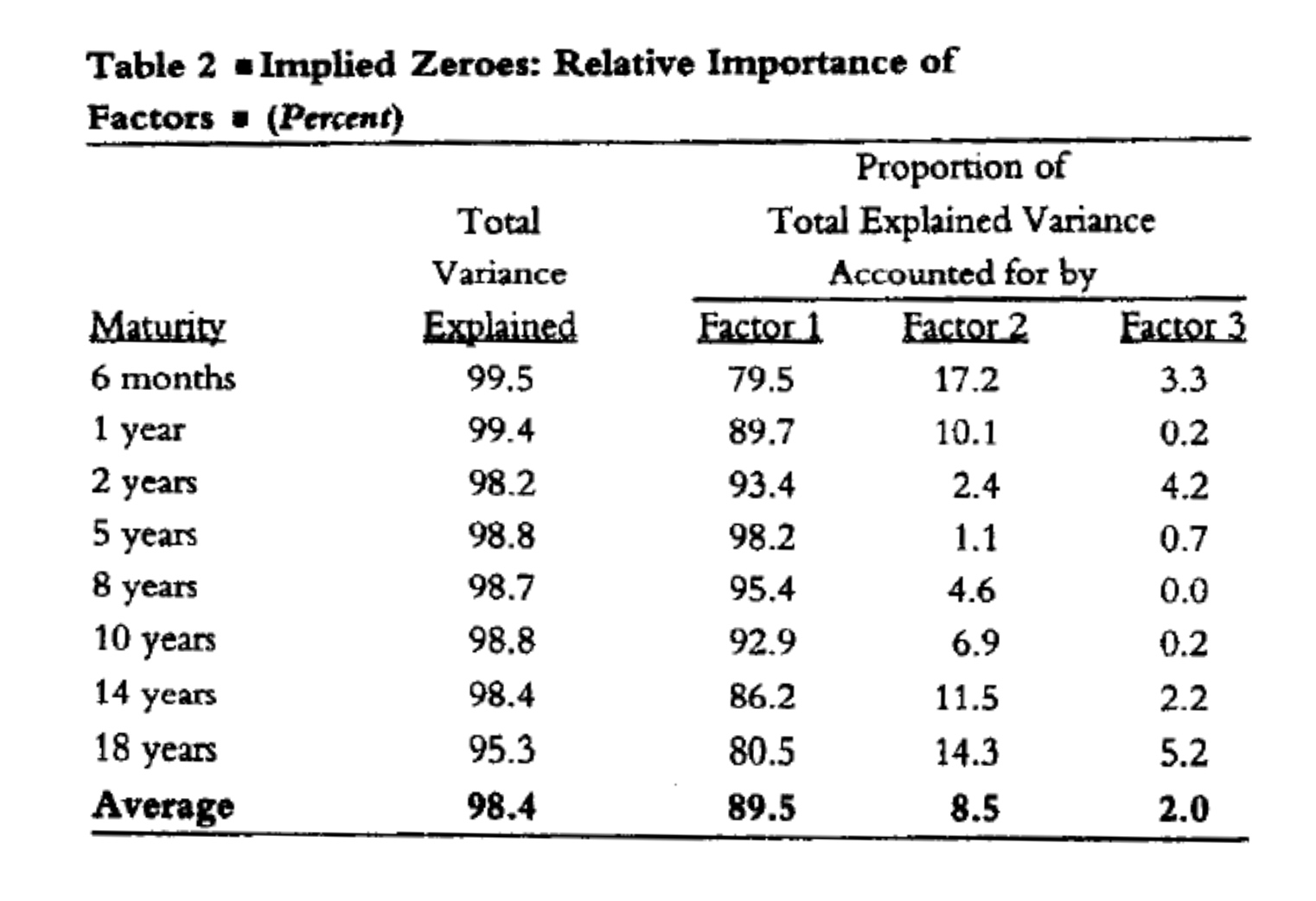
Factor Duration
The Factor Duration with respect to factor j:
\[D_j=-\frac{1}{P}\times \frac{dP}{dF_j}\]Asset returns in a three-factor world:
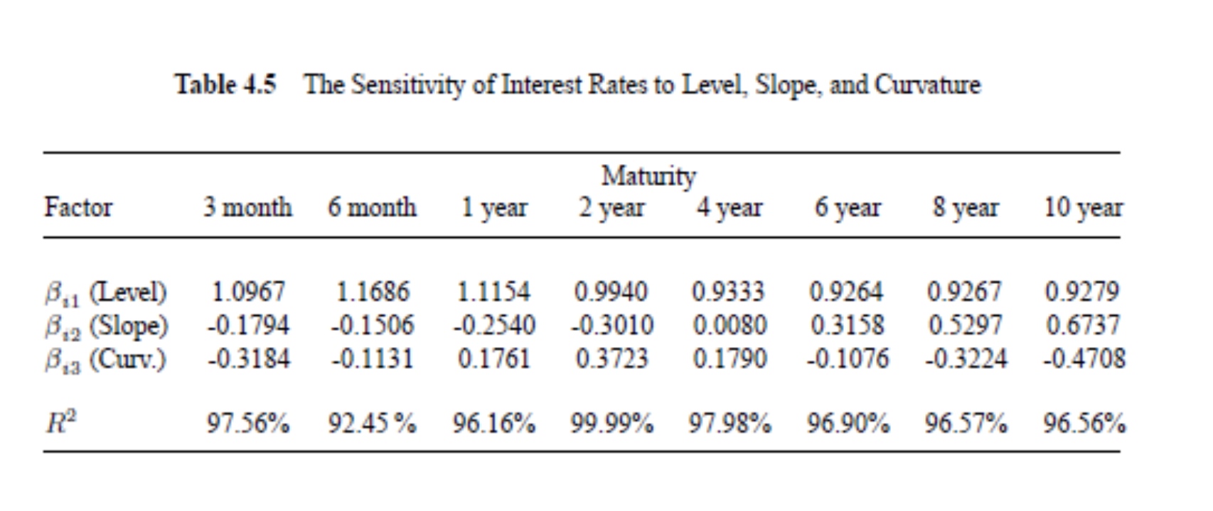
\[\frac{d P}{P}=-D_{1} \times d F_{1}-D_{2} \times d F_{2}-D_{3} \times d F_{3}\]Factor duration for a ZCB
\[D_{j}=-\frac{\frac{d P_{z}}{d F_{j}}}{P_{z}}=-\frac{\frac{d P_{z}}{d r} \times \frac{d r}{d F_{j}}}{P_{z}}=(T-t) \times \frac{d r}{d F_{j}}=(T-t) \times \beta_{j}^{(T)}\]We can use Linear regression or PCA to find the appropriate $\beta_j^T$:
Factor duration for a portfolio
\[V=\sum_{i} P_{i} \Rightarrow D_{V, j}=\sum_{i} w_{i} D_{i, j}\]Applied to fixed coupon bonds:
\[D_j=\sum_i^n w_i (T_i -t) \beta_j^i\]Factor neutrality
Overall portfolio: $V=P+K_S P_S +K_L P_L $
Neutralize portfolio returns:
\[𝑑V= 𝑑𝑃 + 𝑘_S𝑑𝑃_S + 𝑘_L𝑑𝑃_L = 0\]Portfolio returns decomposed:
\[\begin{array}{c} 0=-D_{1} \times P \times d F_{1}-D_{2} \times P \times d F_{2} \\ +k_{S}\left(-D_{S 1} \times P_{S} \times d F_{1}-D_{S 2} \times P_{S} \times d F_{2}\right) \\ +k_{L}\left(-D_{L 1} \times P_{L} \times d F_{1}-D_{L 2} \times P_{L} \times d F_{2}\right) \end{array}\]Portfolio returns, decomposed into factors:
\[\begin{array}{l} 0=-\left(D_{1} \times P+k_{S} \times D_{S 1} \times P_{S}+k_{L} \times D_{L 1} \times P_{L}\right) \times d F_{1} \\ \quad-\left(D_{2} \times P+k_{S} \times D_{S 2} \times P_{S}+k_{L} \times D_{L 2} \times P_{L}\right) \times d F_{2} \end{array}\]Neutrality for both factors requires:
\[\begin{array}{l} D_{1} \times P+k_{S} \times D_{S 1} \times P_{S}+k_{L} \times D_{L 1} \times P_{L}=0 \\ D_{2} \times P+k_{S} \times D_{S 2} \times P_{S}+k_{L} \times D_{L 2} \times P_{L}=0 \end{array}\]Value at Risk
The (100 − 𝛼)%, 𝑇 year Value at Risk of a portfolio is the maximum loss the portfolio can suffer over a 𝑇 year horizon with 𝛼% probability:
\[\text{𝑃𝑟𝑜𝑏(𝐿𝑜𝑠𝑠 > 𝑉𝑎𝑅)} = 𝛼\%\]Loss distribution: $L_T=-(P_T-P_0)$, negative if profit.
Expected Shortfall
Expected Shortfall is the expected loss on a portfolio P over the horizon T conditional on the loss being larger than the $(100 – α)\%$ T VaR:
\[\text{Expected Shortfall}=E[L_T | L_T >VaR]\]Expected shortfall is the average outcome in the shaded area:
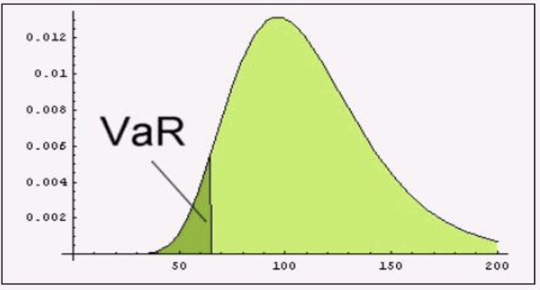
Under normality:
\[\begin{aligned} &95 \% \text { Exp.shortfall }=-\left(\mu-\sigma_{P} \times \frac{f(-1.645)}{N(-1.645)}\right) \\ &=-\left(\mu-\sigma_{P} \times 2.0628\right) \end{aligned}\]where $f(x)$ denotes the standard density and $N(x)$ is the standard normal cumulative density.
Interest Rate Models
Interest rate models in stochastic differential equations (SDEs):
- Ho-Lee model: \(d r_{t}=\theta_{t} d t+\sigma d X_{t}\)
- Varsicek model: \(d r_{t}=\gamma\left(\bar{r}-r_{t}\right) d t+\sigma d X_{t}\)
- Cox-Ingersoll-Ross (CIR) model: \(d r_{t}=\gamma\left(\bar{r}-r_{t}\right) d t+\sigma \sqrt{r_{t}} d X_{t}\)
- Dothan model: \(d r_{t}=\theta r_{t} d t+\sigma r_{t} d X_{t}\)
- Black-Derman-Toy (BDT) model: \(d r_{t}=\theta_{t} r_{t} d t+\sigma_{t} r_{t} d X_{t}\)
- Hull-White (extended Varsicek) model: \(d r_{t}=\gamma_{t}\left(\bar{r}-r_{t}\right) d t+\sigma_{t} d X_{t}\)
Single factor affine models
- An affine process 𝑥’ has the following form
- Both the (instantaneous) drift and variance is affine in $x_{t}$ :
Continuous time Vasicek model
- Discrete time risk-neutral short rate process with time step $\Delta$
- Continuous time Vasicek model is the $\Delta \rightarrow 0$ limit
- Price of ZCBs:
- The solution to system of ODEs is:
- The price at time $t$ of a ZCB with face value 1 and which matures at $T \geq t$ is given by
- Alternately, we can write in terms of time to maturity $\tau \stackrel{\text { def }}{=} T-t \geq 0$
- Then:
where
\[\begin{gathered} A(\tau)=(B(\tau)-\tau)\left(\bar{r}^{*}-\frac{\sigma^{2}}{2\left(\gamma^{*}\right)^{2}}\right)-\frac{\sigma^{2} B(\tau)^{2}}{4 \gamma^{*}} \\ B(\tau)=\frac{1}{\gamma^{*}}\left(1-e^{-\gamma^{*} \tau}\right) \end{gathered}\]- The $\tau$ year yield to maturity is:
- The spot rate duration is:
Cox, Ingersoll, Ross (CIR)
The shortcoming of Vasicek model is that the $r_t$ can be negative.
- CIR models short rate as a “square root process”: \(r_{t+\Delta}=\left(1-\rho_{\Delta}\right) \bar{r}+\rho_{\Delta} r_{t}+\sqrt{\alpha r_{t} \Delta} \varepsilon_{t+\Delta}\)
- Volatility $\sqrt{\alpha r_{t}}$ is no longer constant
- Preserves mean reversion properties
- The long run mean is $\bar{r}$
- There is mean reversion:
- Positive drift if $r_{t}<\bar{r}$
- Negative drift if $r_{t}>\bar{r}$
Price of ZCBs:
Solution is:
\[Z(t, r ; T)=e^{A(t ; T)-B(t ; T) \times r}\]where:
\[\begin{aligned} &B(t ; T)=\frac{2\left(e^{\psi_{1}(T-t)}-1\right)}{\left(\gamma^{*}+\psi_{1}\right)\left(e^{\psi_{1}(T-t)}-1\right)+2 \psi_{1}} \\ &A(t ; T)=2 \frac{\bar{r}^{*} \gamma^{*}}{\alpha} \log \left(\frac{2 \psi_{1} e^{\left(\psi_{1}+\gamma^{*}\right) \frac{(T-t)}{2}}}{\left(\gamma^{*}+\psi_{1}\right)\left(e^{\psi_{1}(T-t)}-1\right)+2 \psi_{1}}\right) \end{aligned}\]and
\[\psi_{1}=\left(\left(\gamma^{*}\right)^{2}+2 \alpha\right)^{1 / 2}\]Calibration
Calibrating the Vasicek model
- Estimate parameters:
- Choose them to minimize pricing errors:
Comments