Machine Learning With Python

This series of Data Science posts are my notes for the IBM Data Science Professional Certificate.

Skills:

• Regression: predicting continuous values
• Classification: predicting the item class of a case
• Clustering: finding the structure of data, summarization
• Associations: associating frequent co-occurring items/events
• Anomaly detection: discovering abnormal and unusual cases
• Sequence mining: predicting next events
• Dimension Reduction: reducing the size of data(PCA)
• Recommendation systems
• Scikit Learn:
• Scipy

Projects:

• Cancer detection
• Predicting economic trends
• Predicting customer churn
• Recommendation Engines
• Many more..

Introduction to Machine Learning

What is machine learning? Machine learning is the subfield of computer science that gives “computers the ability to learn without being explicitly programmed.”

Difference bewteen artificial intelligence, machine learning, and deep learning.

• AI components: AI tries to make computers intelligent in order to mimic the cognitive functions of humans.
  • Computer vision
  • Language processing
  • Creativity
  • Summarization.
• Machine Learning: Machine Learning is the branch of AI that covers the statistical part of artificial intelligence. It teaches the computer to solve problems by looking at hundreds or thousands of examples, learning from them, and then using that experience to solve the same problem in new situations.
  • Classification
  • Clustering
  • Neural Network
• Revolution in ML
  • Deep learning: Deep Learning is a very special field of Machine Learning where computers can actually learn and make intelligent decisions on their own.

Python for Machine Learning

Numpy The first package is NumPy which is a math library to work with N-dimensional arrays in Python. It enables you to do computation efficiently and effectively. It is better than regular Python because of its amazing capabilities

Scipy is a collection of numerical algorithms and domain specific toolboxes, including signal processing, optimization, statistics and much more

Pandas library is a very high-level Python library that provides high performance easy to use data structures. It has many functions for data importing, manipulation and analysis. In particular, it offers data structures and operations for manipulating numerical tables and timeseries.

SciKit Learn is a collection of algorithms and tools for machine learning

Most of the tasks that need to be done in a machine learning pipeline are implemented already in Scikit Learn including pre-processing of data, feature selection, feature extraction, train test splitting, defining the algorithms, fitting models, tuning parameters, prediction, evaluation, and exporting the model.

Supervised vs Unsupervised

Supervised: deal with labeled data

• regression
• classification

Unsupervised: deal with unlabeled data

• dimension reduction
• density estimate
• market basket analysis
• clustering
  • Discovering structure
  • Summarization
  • Anomaly detection

Introduction to Regression

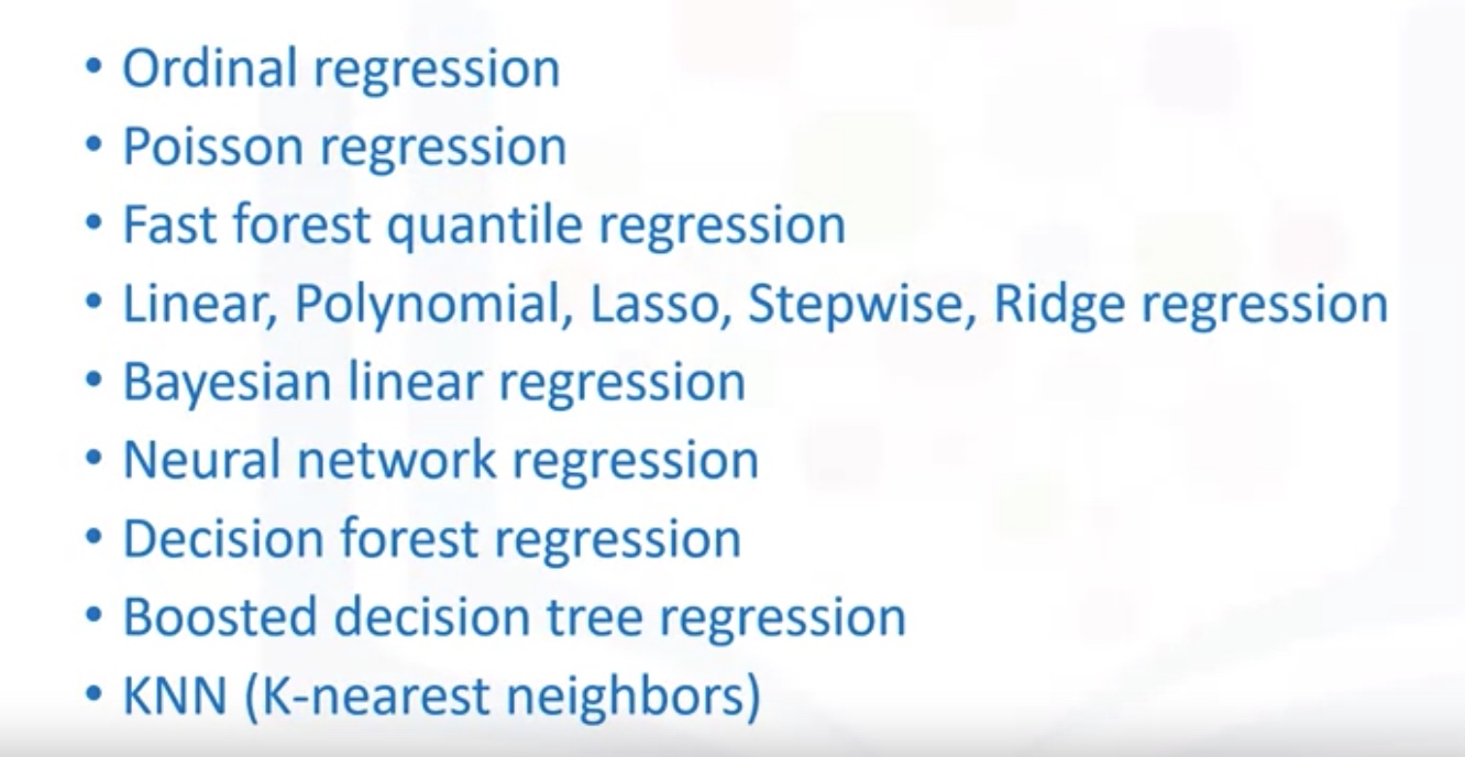
Regression algorithms:

Model Evaluation approaches

• Train and Test on the same Dataset
• Train/Test split
• Regression Evaluation Metrics

Training Accuracy:

• High training accuracy isn’t necessarily a good thing
• Result of over-fitting: the model is overly trained to the dataset, which may capture noise and produce a non-generalized model.

Out-of-sample accuracy

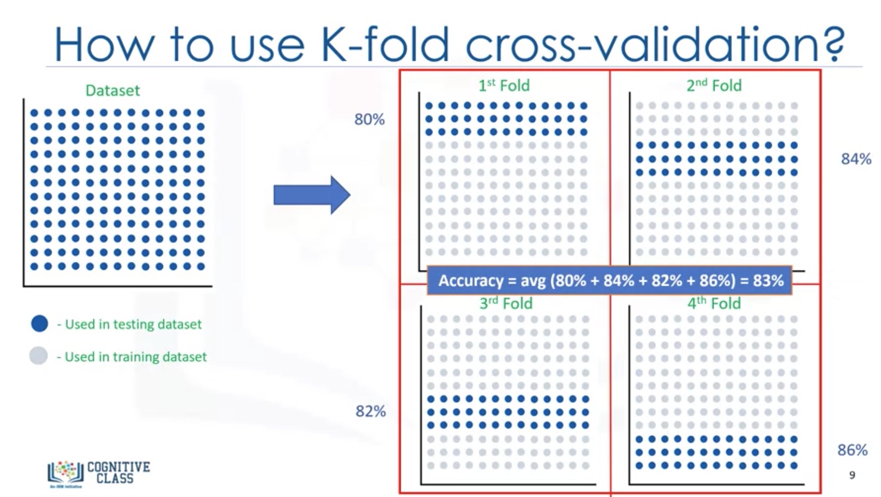
Since the result highly depend on which datasets the data is trained and tested, we better use K-fold cross-validation.

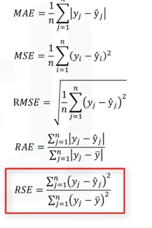
Evaluation Metrics in regression models

• R square：R^2=1-RSE
• MSE: mean square error
• MAE: mean absolute error
• RMES: root of mean square error
• RSE: relative square error

• RAE: relative average error

  

Lab section - Linear Regression

import matplotlib.pyplot as plt
import pandas as pd
import pylab as pl
import numpy as np
%matplotlib inline

!wget -O FuelConsumption.csv https://s3-api.us-geo.objectstorage.softlayer.net/cf-courses-data/CognitiveClass/ML0101ENv3/labs/FuelConsumptionCo2.csv

df = pd.read_csv("FuelConsumption.csv")

# use color map to see the correlation
cdf = df[['ENGINESIZE','CYLINDERS','FUELCONSUMPTION_COMB','CO2EMISSIONS']]
cdf.head(9)
cdf.corr()
plt.pcolor(cdf.corr())
plt.colorbar()
plt.show()

# scatter plot
plt.scatter(cdf.FUELCONSUMPTION_COMB, cdf.CO2EMISSIONS,  color='blue')
plt.xlabel("FUELCONSUMPTION_COMB")
plt.ylabel("Emission")
plt.show()


# Lets split our dataset into train and test sets, 80% of the entire data for training, and the 20% for testing. We create a mask to select random rows using np.random.rand() function:

msk = np.random.rand(len(df)) < 0.8
train = cdf[msk]
test = cdf[~msk]

# Train Data Distribution
plt.scatter(train.ENGINESIZE, train.CO2EMISSIONS,  color='blue')
plt.xlabel("Engine size")
plt.ylabel("Emission")
plt.show()

# modeling with sklearn package
from sklearn import linear_model
lr=linear_model.LinearRegression()
# Note the X must be a matrix, and must use [['col_Xs']]
lr.fit(train[['ENGINESIZE']],train['CO2EMISSIONS'])
lr.coef_
lr.intercept_


# plot output
train_X=train[['ENGINESIZE']]
plt.scatter(train.ENGINESIZE, train.CO2EMISSIONS,  color='blue')
plt.plot(train_X, lr.predict(train_X), '-r')
plt.xlabel("Engine size")
plt.ylabel("Emission")

# Evaluation
lr.score(test[['ENGINESIZE']], test.CO2EMISSIONS)

# or use r2_score for non-linear regression
from sklearn.metrics import r2_score

test_x = np.asanyarray(test[['ENGINESIZE']])
test_y = np.asanyarray(test[['CO2EMISSIONS']])
test_y_hat = lr.predict(test_x)

print("Mean absolute error: %.2f" % np.mean(np.absolute(test_y_hat - test_y)))
print("Residual sum of squares (MSE): %.2f" % np.mean((test_y_hat - test_y) ** 2))
print("R2-score: %.2f" % r2_score(test_y_hat , test_y) )


# Note that, r2_socre(y_hat, y_real)

Non-Linear Regression

It is important to pick a regression model that fits the data the best.

How should I model my data, if it displays non-linear on a scatter plot?

• Polynomial regression
• Non-Linear regression model
• transform the data

Lab: Polynomial regression

from sklearn.preprocessing import PolynomialFeatures
from sklearn import linear_model
train_x = np.asanyarray(train[['ENGINESIZE']])
train_y = np.asanyarray(train[['CO2EMISSIONS']])

test_x = np.asanyarray(test[['ENGINESIZE']])
test_y = np.asanyarray(test[['CO2EMISSIONS']])


poly = PolynomialFeatures(degree=2)
train_x_poly = poly.fit_transform(train_x)
train_x_poly

clf = linear_model.LinearRegression()
clf.fit(train_x_poly, train_y)
# The coefficients
print ('Coefficients: ', clf.coef_)
print ('Intercept: ',clf.intercept_)


# Print the output
plt.scatter(train.ENGINESIZE, train.CO2EMISSIONS,  color='blue')
XX = np.arange(0.0, 10.0, 0.1)
# Note that we only accept the matrix as input for the predcit and fit function! Better use reshape(-1,1)
yy = clf.predict(poly.fit_transform(XX.reshape(-1,1)))
plt.plot(XX, yy, '-r' )
plt.xlabel("Engine size")
plt.ylabel("Emission")

# Evaluation
from sklearn.metrics import r2_score
test_x_poly = poly.fit_transform(test_x)
test_y_ = clf.predict(test_x_poly)

print("Mean absolute error: %.2f" % np.mean(np.absolute(test_y_ - test_y)))
print("Residual sum of squares (MSE): %.2f" % np.mean((test_y_ - test_y) ** 2))
print("R2-score: %.2f" % r2_score(test_y_ , test_y) )

Lab: Non-linear regression analysis

import numpy as np
import matplotlib.pyplot as plt
%matplotlib inline

x = np.arange(-5.0, 5.0, 0.1)

##You can adjust the slope and intercept to verify the changes in the graph
y = 2*(x) + 3
y_noise = 2 * np.random.normal(size=x.size)
ydata = y + y_noise
#plt.figure(figsize=(8,6))
plt.plot(x, ydata,  'bo')
plt.plot(x,y, 'r')
plt.ylabel('Dependent Variable')
plt.xlabel('Indepdendent Variable')
plt.show()

Non-linear regressions are a relationship between independent variables $x$ and a dependent variable $y$ which result in a non-linear function modeled data. Essentially any relationship that is not linear can be termed as non-linear, and is usually represented by the polynomial of $k$ degrees (maximum power of $x$).

\[\ y = a x^3 + b x^2 + c x + d \\]

Non-linear functions can have elements like exponentials, logarithms, fractions, and others. For example: \(y = \log(x)\)

Or even, more complicated such as :

\[y = \log(a x^3 + b x^2 + c x + d)\]

Non-linear regression example

import numpy as np
import pandas as pd

#downloading dataset
!wget -nv -O china_gdp.csv https://s3-api.us-geo.objectstorage.softlayer.net/cf-courses-data/CognitiveClass/ML0101ENv3/labs/china_gdp.csv

df = pd.read_csv("china_gdp.csv")
df.head(10)

# plot the data
plt.figure(figsize=(8,5))
x_data, y_data = (df["Year"].values, df["Value"].values)
plt.plot(x_data, y_data, 'ro')
plt.ylabel('GDP')
plt.xlabel('Year')
plt.show()

# choosing a model
X = np.arange(-5.0, 5.0, 0.1)
Y = 1.0 / (1.0 + np.exp(-X))

plt.plot(X,Y)
plt.ylabel('Dependent Variable')
plt.xlabel('Indepdendent Variable')
plt.show()

The formula for the logistic function is the following:

\[\hat{Y} = \frac1{1+e^{-\beta_1(X-\beta_2)}}\]

$\beta_1$: Controls the curve’s steepness,

$\beta_2$: Slides the curve on the x-axis.

def sigmoid(x, Beta_1, Beta_2):
    y = 1 / (1 + np.exp(-Beta_1*(x-Beta_2)))
    return y

beta_1 = 0.10
beta_2 = 1990.0

#logistic function
Y_pred = sigmoid(x_data, beta_1 , beta_2)

#plot initial prediction against datapoints
plt.plot(x_data, Y_pred*15000000000000.)
plt.plot(x_data, y_data, 'ro')


# find the best parameters
# Lets normalize our data
xdata =x_data/max(x_data)
ydata =y_data/max(y_data)

How we find the best parameters for our fit line? we can use curve_fit which uses non-linear least squares to fit our sigmoid function, to data. Optimal values for the parameters so that the sum of the squared residuals of sigmoid(xdata, *popt) - ydata is minimized.

popt are our optimized parameters.

from scipy.optimize import curve_fit
popt, pcov = curve_fit(sigmoid, xdata, ydata)
#print the final parameters
print(" beta_1 = %f, beta_2 = %f" % (popt[0], popt[1]))

# Now plot the output
x = np.linspace(1960, 2015, 55)
x = x/max(x)
plt.figure(figsize=(8,5))
y = sigmoid(x, *popt)
plt.plot(xdata, ydata, 'ro', label='data')
plt.plot(x,y, linewidth=3.0, label='fit')
plt.legend(loc='best')
plt.ylabel('GDP')
plt.xlabel('Year')
plt.show()


# evaluation
from sklearn.metrics import r2_score
# split data into train/test
msk = np.random.rand(len(df)) < 0.8
train_x = xdata[msk]
test_x = xdata[~msk]
train_y = ydata[msk]
test_y = ydata[~msk]

# build the model using train set
popt, pcov = curve_fit(sigmoid, train_x, train_y)

# predict using test set
y_hat = sigmoid(test_x, *popt)

# Finally we have the following result:
print("Mean absolute error: %.2f" % np.mean(np.absolute(y_hat - test_y)))
print("Residual sum of squares (MSE): %.2f" % np.mean((y_hat - test_y) ** 2))
from sklearn.metrics import r2_score
print("R2-score: %.2f" % r2_score(test_y, y_hat) )

Introduction to Classification

Classification algorithms in machine learning:

• Decision Trees
• Naive Bayes
• Linear Discriminant Analysis
• K-nearest Neighbor
• Logistic Regression
• Neural Networks
• Support Vector Machines (SVM)

K-Nearest Neighbors

Supervised Learning case

1. Pick a value for K
2. Calculate the distance of unknown case from all cases.
3. Select the K-observations in the training data that are ‘nearest’ the unknown data point.
4. Predict the response of the unknown data point using the most popular response value from the K-nearest neighbors.

K=1: overfitting. K too big: high train error Plot accuracy VS K: find the optimal K.

Lab: KNN

import itertools
import numpy as np
import matplotlib.pyplot as plt
from matplotlib.ticker import NullFormatter
import pandas as pd
import numpy as np
import matplotlib.ticker as ticker
from sklearn import preprocessing
%matplotlib inline

# Load Data
df = pd.read_csv('teleCust1000t.csv')
df.head()
df.hist(column='income', bins=50)

X = df[['region', 'tenure','age', 'marital', 'address', 'income', 'ed', 'employ','retire', 'gender', 'reside']] .values  #.astype(float)
X[0:5]
y = df['custcat'].values
y[0:5]


# Preprocess Data
# Normalize Data
X = preprocessing.StandardScaler().fit(X).transform(X.astype(float))
X[0:5]

# Train Test Split
from sklearn.model_selection import train_test_split
X_train, X_test, y_train, y_test = train_test_split( X, y, test_size=0.2, random_state=4)
print ('Train set:', X_train.shape,  y_train.shape)
print ('Test set:', X_test.shape,  y_test.shape)

# Train data
from sklearn.neighbors import KNeighborsClassifier
k = 6
#Train Model and Predict
neigh = KNeighborsClassifier(n_neighbors = k).fit(X_train,y_train)
neigh
yhat = neigh.predict(X_test)
yhat[0:5]

# Evaluation
from sklearn import metrics
print("Train set Accuracy: ", metrics.accuracy_score(y_train, neigh.predict(X_train)))
print("Test set Accuracy: ", metrics.accuracy_score(y_test, yhat))


# Plot accuracy VS K

Ks = 10
mean_acc = np.zeros((Ks-1))
std_acc = np.zeros((Ks-1))
ConfustionMx = [];
for n in range(1,Ks):

    #Train Model and Predict
    neigh = KNeighborsClassifier(n_neighbors = n).fit(X_train,y_train)
    yhat=neigh.predict(X_test)
    mean_acc[n-1] = metrics.accuracy_score(y_test, yhat)


    std_acc[n-1]=np.std(yhat==y_test)/np.sqrt(yhat.shape[0])

mean_acc

plt.plot(range(1,Ks),mean_acc,'g')
plt.fill_between(range(1,Ks),mean_acc - 1 * std_acc,mean_acc + 1 * std_acc, alpha=0.10)
plt.legend(('Accuracy ', '+/- 3xstd'))
plt.ylabel('Accuracy ')
plt.xlabel('Number of Nabors (K)')
plt.tight_layout()
plt.show()

Evaluation metrics in classification

Jaccard index: $\begin{equation} J(y, \hat{y})=\frac{|y \cap \hat{y}|}{|y \cup \hat{y}|}=\frac{|y \cap \hat{y}|}{|y|+|\hat{y}|-|y \cap \hat{y}|} \end{equation}$

F1-score

• Precision = TP/(TP+FP)
• Recall = TP/(TP+FN)
• $F1-score= \frac{2PreRec}{(Pre+Rec)}$

$F_1 ~ Score=2 \frac{PR}{P+R}$

Log loss The cost function for logistic regression:

\[\begin{array}{ll}{J(\theta)=\frac{1}{m} \sum_{i=1}^{m} \operatorname{cost}\left(h_{\theta}\left(x^{(i)}\right), y^{(i)}\right)} \\ {\operatorname{Cost}\left(h_{\theta}(x), y\right)=-\log \left(h_{\theta}(x)\right)} & {\text { if } y=1} \\ {\operatorname{Cost}\left(h_{\theta}(x), y\right)=-\log \left(1-h_{\theta}(x)\right)} & {\text { if } y=0}\end{array}\]

Log loss: $\begin{equation} \text { LogLoss }=-\frac{1}{n} \sum[y \times \log (\hat{y})+(1-y) \times \log (1-\hat{y})] \end{equation}$

where: y is the actual value, $\hat{y}$ is the predicted value.

Decisions Tress

Algorithm:

1. Choose an attribute from your dataset
2. Calculate the significance of attribute in splitting of data
3. Split data based on the value of the best attribute
4. Go to step 1

Apparently, the most import step in decision tree model is to find the best attribute.

Entropy: measure of randomness or uncertainty. The lower the Entropy, the less uniform the distribution, the purer the node.

\[Entropy=-p(A)log_2 (p(A))-p(B)log_2 (p(B))\]

Which Attribute? -> The Tree with the higher information gain after splitting.

Information gain is the information tha can increase the level of certainty after splitting.

$information gain = \text{Entropy before split} - \text{Weighted Entropy after split}$

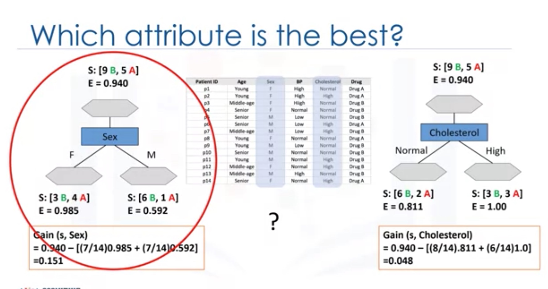
we then repeat the process for each branch to reach the most pure leaves.

\[Entropy=-p(A)log_2 (p(A))-p(B)log_2 (p(B))\]

Given a random variable ${\displaystyle X}$, with possible outcomes ${\displaystyle x_{i}}$, each with probability ${\displaystyle P_{X}(x_{i})}$, the entropy ${\displaystyle H(X)}$ of ${\displaystyle X}$ is as follows:

\[H(X)=-\sum _{i}P_{X}(x_{i})\log _{b}{P_{X}(x_{i})}=\sum _{i}P_{X}(x_{i})I_{X}(x_{i})=\operatorname {E} [I_{X}]\]

where ${\displaystyle I_{X}(x_{i})}$ is the self-information associated with particular outcome; ${\displaystyle I_{X}}$ is the self-information of the random variable X in general, treated as a new derived random variable; and ${\displaystyle \operatorname {E} [I_{X}]}$ is the expected value of this new random variable, equal to the sum of the self-information of each outcome, weighted by the probability of each outcome occurring[3]; and b, the base of the logarithm, is a new parameter that can be set different ways to determine the choice of units for information entropy.

Information entropy is typically measured in bits (alternatively called “shannons”), corresponding to base 2 in the above equation. It is also sometimes measured in “natural units” (nats), corresponding to base e, or decimal digits (called “dits”, “bans”, or “hartleys”), corresponding to base 10.

Lab: DecisionTreeClassifier

import numpy as np
import pandas as pd
from sklearn.tree import DecisionTreeClassifier

#Load Data
my_data = pd.read_csv("drug200.csv", delimiter=",")

# Preprocessing

X = my_data[['Age', 'Sex', 'BP', 'Cholesterol', 'Na_to_K']].values
X[0:5]

from sklearn import preprocessing
le_sex = preprocessing.LabelEncoder()
le_sex.fit(['F','M'])
X[:,1] = le_sex.transform(X[:,1])


le_BP = preprocessing.LabelEncoder()
le_BP.fit([ 'LOW', 'NORMAL', 'HIGH'])
X[:,2] = le_BP.transform(X[:,2])


le_Chol = preprocessing.LabelEncoder()
le_Chol.fit([ 'NORMAL', 'HIGH'])
X[:,3] = le_Chol.transform(X[:,3])

y = my_data["Drug"]

#Split the data
from sklearn.model_selection import train_test_split
X_trainset, X_testset, y_trainset, y_testset = train_test_split(X, y, test_size=0.3, random_state=3)


# Train the model
drugTree = DecisionTreeClassifier(criterion="entropy", max_depth = 4)
drugTree # it shows the default parameters

drugTree.fit(X_trainset,y_trainset)

predTree = drugTree.predict(X_testset)

# Evaluation
from sklearn import metrics
import matplotlib.pyplot as plt
print("DecisionTrees's Accuracy: ", metrics.accuracy_score(y_testset, predTree))

Logistic Regression

While Linear Regression is suited for estimating continuous values (e.g. estimating house price), it is not the best tool for predicting the class of an observed data point. In order to estimate the class of a data point, we need some sort of guidance on what would be the most probable class for that data point. For this, we use Logistic Regression.

Recall linear regression: As you know, Linear regression finds a function that relates a continuous dependent variable, y to some predictors (independent variables $x_1$, $x_2$, etc.). For example, Simple linear regression assumes a function of the form:

\[y = \theta_0 + \theta_1 x_1 + \theta_2 x_2 + \cdots\]

and finds the values of parameters $\theta_0, \theta_1, \theta_2$, etc, where the term $\theta_0$ is the “intercept”. It can be generally shown as:

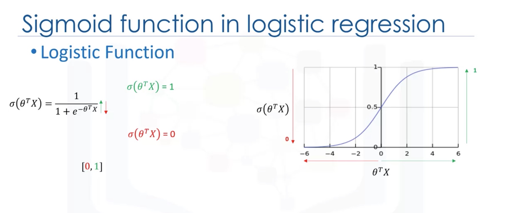
\[ℎ_\theta(𝑥) = \theta^TX\]

Logistic Regression is a variation of Linear Regression, useful when the observed dependent variable, y, is categorical. It produces a formula that predicts the probability of the class label as a function of the independent variables.

Logistic regression fits a special s-shaped curve by taking the linear regression and transforming the numeric estimate into a probability with the following function, which is called sigmoid function 𝜎:

\[ℎ_\theta(𝑥) = \sigma({\theta^TX}) = \frac {e^{(\theta_0 + \theta_1 x_1 + \theta_2 x_2 +...)}}{1 + e^{(\theta_0 + \theta_1 x_1 + \theta_2 x_2 +\cdots)}}\]

Or:

\[ProbabilityOfaClass_1 = P(Y=1|X) = \sigma({\theta^TX}) = \frac{e^{\theta^TX}}{1+e^{\theta^TX}}\]

In this equation, ${\theta^TX}$ is the regression result (the sum of the variables weighted by the coefficients), exp is the exponential function and $\sigma(\theta^TX)$ is the sigmoid or logistic function, also called logistic curve. It is a common “S” shape (sigmoid curve).

So, briefly, Logistic Regression passes the input through the logistic/sigmoid but then treats the result as a probability:

The objective of Logistic Regression algorithm, is to find the best parameters θ, for $ℎ_\theta(𝑥)$ = $\sigma({\theta^TX})$, in such a way that the model best predicts the class of each case.

Algorithm:

1. Initialize $\theta$
2. calculate $\hat{y}=g(\theta^T X)$ for a customer
3. get the cost function
4. optimize the cost function over $\theta$

\[\begin{aligned} J(\theta) &=\frac{1}{m} \sum_{i=1}^{m} \operatorname{cost}\left(h_{\theta}\left(x^{(i)}\right), y^{(i)}\right) \\ &=-\frac{1}{m}\left[\sum_{i=1}^{m} y^{(i)} \log h_{\theta}\left(x^{(i)}\right)+\left(1-y^{(i)}\right) \log \left(1-h_{\theta}\left(x^{(i)}\right)\right)\right] \end{aligned}\]

Which is still convex function.

Proposition about convex functions

• If $f(\cdot)$ is convex function, $g(\cdot)$ is an linear/affine function, then $f(g(\cdot))$ is a convex function.
• If $f(\cdot)$ and $g(\cdot)$ are both convex function, then $af(x)+bg(y)$ is still convex function if $a,b>=0$.

Essentially, $Cost~function \in [0,+\infty )$

• $Cost~function \to +\infty$ if $

  h_\theta(x)-y

  \to 1 $.

• $Cost~function \to 0$ if $

  h_\theta(x)-y

  \to 0 $.

Note that writing the cost function in this way guarantees that $J(\theta )$ is convex for logistic regression.

Gradient Descent

\[\begin{array}{l}{\text { Gradient Descent }} \\ {\qquad \begin{array}{l}{J(\theta)=-\frac{1}{m}\left[\sum_{i=1}^{m} y^{(i)} \log h_{\theta}\left(x^{(i)}\right)+\left(1-y^{(i)}\right) \log \left(1-h_{\theta}\left(x^{(i)}\right)\right)\right]} \\ {\text { Want } \min _{\theta} J(\theta) :} \\ {\text { Repeat }\{ } \end{array}} \\ {\qquad \begin{array}{ll} {\theta_{j} :=\theta_{j}-\alpha \frac{\partial}{\partial \theta_{j}} J(\theta)} \\ { \}} & {\left.\text { (simultaneously update all } \theta_{j}\right)}\end{array}}\end{array}\]

Since $\frac{\partial} {\partial \theta_j} J(\theta)=\frac{1}{m}\sum_{i=1}^m(h_\theta(x^{(i)})-y^{(i)})x_j^{(i)}$, we get:

\[\begin{array}{l}{\text { Gradient Descent }} \\ {\qquad \begin{array}{l}{J(\theta)=-\frac{1}{m}\left[\sum_{i=1}^{m} y^{(i)} \log h_{\theta}\left(x^{(i)}\right)+\left(1-y^{(i)}\right) \log \left(1-h_{\theta}\left(x^{(i)}\right)\right)\right]} \\ {\text { Want } \min _{\theta} J(\theta) :} \\ {\text { Repeat }\{ } \end{array}} \\ {\qquad \begin{array}{ll} {\theta_{j} :=\theta_{j}-\frac{\alpha}{m} \sum_{i=1}^m(h_\theta(x^{(i)})-y^{(i)})x_j^{(i)}} \\ { \}} & {\left.\text { (simultaneously update all } \theta_{j}\right)}\end{array}}\end{array}\]

Vectorization

Use the built in functions to solve the calculation. Try not to implement the loop by ourselves.

For example, in the gradient descent method, we need to calculate simultaneously:

\[\begin{array}{l}{\text { repeat until convergence: } } \\ {\theta_{j} :=\theta_{j}-\alpha \frac{1}{m} \sum_{i=1}^{m}\left(h_{\theta}\left(x^{(i)}\right)-y^{(i)}\right) \cdot x_{j}^{(i)} \quad \text { for } j :=0 \ldots n}\end{array}\]

In fact, this is equivalent to:

$\theta_{new}=\theta-\frac{\alpha}{m}X^T[g(X\theta)-y)]$

Lab: logistic regression

import pandas as pd
import pylab as pl
import numpy as np
import scipy.optimize as opt
from sklearn import preprocessing
%matplotlib inline
import matplotlib.pyplot as plt

churn_df = pd.read_csv("ChurnData.csv")
churn_df.head()

# Data pre-processing and selection
churn_df = churn_df[['tenure', 'age', 'address', 'income', 'ed', 'employ', 'equip',  'callcard', 'wireless','churn']]
churn_df['churn'] = churn_df['churn'].astype('int')
churn_df.head()

X = np.asarray(churn_df[['tenure', 'age', 'address', 'income', 'ed', 'employ', 'equip']])
X[0:5]

y = np.asarray(churn_df['churn'])
y [0:5]

# Normalize the dataset
from sklearn import preprocessing
X = preprocessing.StandardScaler().fit(X).transform(X)
X[0:5]

# Split the test and train set
from sklearn.model_selection import train_test_split
X_train, X_test, y_train, y_test = train_test_split( X, y, test_size=0.2, random_state=4)
print ('Train set:', X_train.shape,  y_train.shape)
print ('Test set:', X_test.shape,  y_test.shape)

# Training
from sklearn.linear_model import LogisticRegression
from sklearn.metrics import confusion_matrix
LR = LogisticRegression(C=0.01, solver='liblinear').fit(X_train,y_train)
LR

yhat = LR.predict(X_test)
yhat

yhat_prob = LR.predict_proba(X_test)
yhat_prob

# __predict_proba__  returns estimates for all classes, ordered by the label of classes. So, the first column is the probability of class 1, P(Y=1|X), and second column is probability of class 0, P(Y=0|X):

# Evaluation
from sklearn.metrics import jaccard_similarity_score
jaccard_similarity_score(y_test, yhat)

# Confusion matrix
print (classification_report(y_test, yhat))

# log loss
from sklearn.metrics import log_loss
log_loss(y_test, yhat_prob)

Support Vector Machine

SVM is a supervised algorithm that classifies cases by finding a separator.

1. Mapping data to a high-dimensional feature spaces.
2. Finding a separator.

Data Transformation

Basically, mapping data into a dimensional space is called Kernelling. The mathematical function which is used for the transformation is called the kernel function.

• Linear
• Polynomial
• RBF
• Sigmoid

Using SVM to find the hyperplane

Pros and Cons of SVM

• Advantages:

  • Accurate in high-dimensional spaces
  • Memory efficient.(only use support vectors)

• Disadvantages:

  • Prone to over-fitting
  • No probability estimation
  • Small datasets

  SVM Applications: (works well with high-dimensional data)

  • Image recognition
  • Text category assignment
  • Detecting spam
  • Sentiment analysis
  • Gene expression classiciation
  • regression, outlier detection and clustering.

LAB: svm

import pandas as pd
import pylab as pl
import numpy as np
import scipy.optimize as opt
from sklearn import preprocessing
from sklearn.model_selection import train_test_split
%matplotlib inline
import matplotlib.pyplot as plt

cell_df = pd.read_csv("cell_samples.csv")
cell_df.head()

# Plot the distribution of the classes:
# Note: when plot composite of axes, use the "label=" parameter to differentiate between different draws.
ax = cell_df[cell_df['Class'] == 4][0:50].plot(kind='scatter', x='Clump', y='UnifSize', color='DarkBlue', label='malignant');
cell_df[cell_df['Class'] == 2][0:50].plot(kind='scatter', x='Clump', y='UnifSize', color='Yellow', label='benign', ax=ax);
plt.show()

# Preprocessing
# convert BareNuc into numerical dtypes
cell_df = cell_df[pd.to_numeric(cell_df['BareNuc'], errors='coerce').notnull()]
cell_df['BareNuc'] = cell_df['BareNuc'].astype('int')
cell_df.dtypes

feature_df = cell_df[['Clump', 'UnifSize', 'UnifShape', 'MargAdh', 'SingEpiSize', 'BareNuc', 'BlandChrom', 'NormNucl', 'Mit']]
X = np.asarray(feature_df)
X[0:5]

cell_df['Class'] = cell_df['Class'].astype('int')
y = np.asarray(cell_df['Class'])
y [0:5]

# Train/Test Split
X_train, X_test, y_train, y_test = train_test_split( X, y, test_size=0.2, random_state=4)
print ('Train set:', X_train.shape,  y_train.shape)
print ('Test set:', X_test.shape,  y_test.shape)

The SVM algorithm offers a choice of kernel functions for performing its processing. Basically, mapping data into a higher dimensional space is called kernelling. The mathematical function used for the transformation is known as the kernel function, and can be of different types, such as:

1. Linear
2. Polynomial
3. Radial basis function (RBF)
4. Sigmoid

# Training/Modeling
from sklearn import svm
clf = svm.SVC(kernel='rbf')
clf.fit(X_train, y_train)

from sklearn import svm
clf = svm.SVC(kernel='rbf')
clf.fit(X_train, y_train)


yhat = clf.predict(X_test)
yhat [0:5]

# Evaluation
from sklearn.metrics import classification_report, confusion_matrix
import itertools

def plot_confusion_matrix(cm, classes,
                          normalize=False,
                          title='Confusion matrix',
                          cmap=plt.cm.Blues):
    """
    This function prints and plots the confusion matrix.
    Normalization can be applied by setting `normalize=True`.
    """
    if normalize:
        cm = cm.astype('float') / cm.sum(axis=1)[:, np.newaxis]
        print("Normalized confusion matrix")
    else:
        print('Confusion matrix, without normalization')

    print(cm)

    plt.imshow(cm, interpolation='nearest', cmap=cmap)
    plt.title(title)
    plt.colorbar()
    tick_marks = np.arange(len(classes))
    plt.xticks(tick_marks, classes, rotation=45)
    plt.yticks(tick_marks, classes)

    fmt = '.2f' if normalize else 'd'
    thresh = cm.max() / 2.
    for i, j in itertools.product(range(cm.shape[0]), range(cm.shape[1])):
        plt.text(j, i, format(cm[i, j], fmt),
                horizontalalignment="center",
                color="white" if cm[i, j] > thresh else "black")

    plt.tight_layout()
    plt.ylabel('True label')
    plt.xlabel('Predicted label')


# Compute confusion matrix
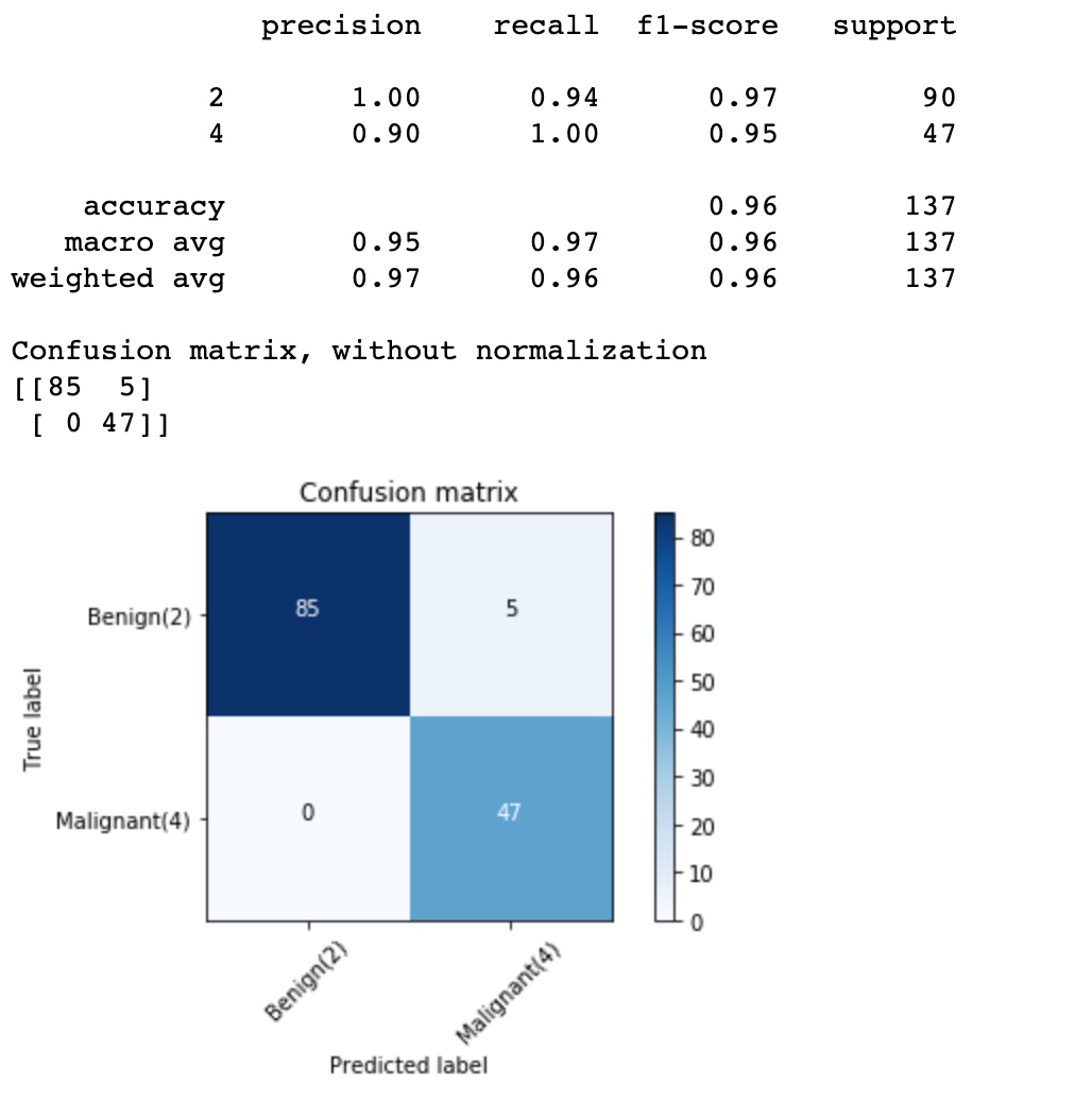
cnf_matrix = confusion_matrix(y_test, yhat, labels=[2,4])
np.set_printoptions(precision=2)

print (classification_report(y_test, yhat))

# Plot non-normalized confusion matrix
plt.figure()
plot_confusion_matrix(cnf_matrix, classes=['Benign(2)','Malignant(4)'],normalize= False,  title='Confusion matrix')

# Other Evaluation
# f1_score
from sklearn.metrics import f1_score
f1_score(y_test, yhat, average='weighted')

# Jaccard index
from sklearn.metrics import jaccard_similarity_score
jaccard_similarity_score(y_test, yhat)

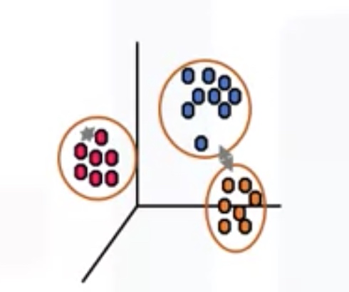
Intro to Clustering

Applications:

• Retail/Marketing

  • Identifying buying patterns of customers
  • Recommending new books or movies to new customers

• Banking

  • Fraud detection in credit card use
  • Identifying clusters of customers
• Insurance
  • Fraud detection in claim analysis
  • Insurance risk of customers

• Publication:

  • Auto-categorizing news based on their content
  • Recommending similar news articles

• Medicine

  • Characterizing patient behavior
• Biology
  • Group genes

Why clustering?

• Exploratory data analysis
• Summary generation
• Outlier detection
• Finding duplicates
• Pre-processing step

Algorithms:

• Partition-based clustering _ Relatively efficient _ K-means, K-median, Fuzzy C-Means

  

• Hierarchical clustering: very intuitive and generally good for small size of data set. _ Produces trees of clusters _ Agglomerative, divisive

  

• Density-based clustering: especially good when dealing spacial clusters or when there is noise in the data set.

  • Produces arbitrary shaped clusters
  • e.g.: DBSCAN

K-means clustering

It is an Unsupervised Learning algorithm.

\[\begin{array}{l}{J\left(c^{(1)}, \ldots, c^{(m)}, \mu_{1}, \ldots, \mu_{K}\right)=\frac{1}{m} \sum_{i=1}^{m}\left\|x^{(i)}-\mu_{c^{(i)}}\right\|^{2}} \\ {\min _{c^{(1)}, \ldots, c^{(m)}} J\left(c^{(1)}, \ldots, c^{(m)}, \mu_{1}, \ldots, \mu_{K}\right)} \\ {\mu_{1}, \ldots, \mu_{K}}\end{array}\]

where $\begin{aligned} c^{(i)} &=\text { index of cluster }(1,2, \ldots, K) \text { to which example } x^{(i)} \text { is currently } \ & \text { assigned } \ \mu_{k} &=\text { cluster centroid } k\left(\mu_{k} \in \mathbb{R}^{n}\right) \end{aligned}$

$\begin{aligned} \mu_{c^{(i)}} &=\text { cluster centroid of cluster to which example } x^{(i)} \text { has been } \ & \text { assigned } \end{aligned}$

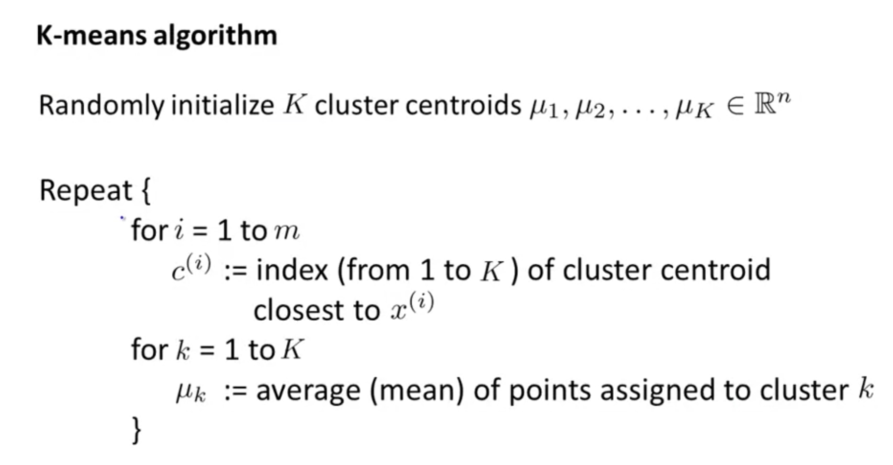
Choose K s.t. the mean distance of data points to cluster centroid is acceptable.

The cost function (distance of data points to the appointed cluster centroid) decreases as K increases. Elbow point is determined where the rate of decrease sharply shifts.

Lab: K-means

Lets create the data set for this lab. First we need to set up a random seed. Use numpy’s random.seed() function, where the seed will be set to 0.

Next we will be making random clusters of points by using the make_blobs class. The make_blobs class can take in many inputs, but we will be using these specific ones.

Input

• n_samples: The total number of points equally divided among clusters.

• • Value will be: 5000

• centers: The number of centers to generate, or the fixed center locations.

• • Value will be: [[4, 4], [-2, -1], [2, -3],[1,1]]

• cluster_std: The standard deviation of the clusters.

• • Value will be: 0.9

Output

• X: Array of shape [n_samples, n_features]. (Feature Matrix)

• • The generated samples.

• y: Array of shape [n_samples]. (Response Vector)

• • The integer labels for cluster membership of each sample.

import random
import numpy as np
import matplotlib.pyplot as plt
from sklearn.cluster import KMeans
from sklearn.datasets.samples_generator import make_blobs
%matplotlib inline

np.random.seed(0)
X, y = make_blobs(n_samples=5000, centers=[[4,4], [-2, -1], [2, -3], [1, 1]], cluster_std=0.9)
plt.scatter(X[:, 0], X[:, 1], marker='.')

The KMeans class has many parameters that can be used, but we will be using these three:

• init: Initialization method of the centroids.

• • Value will be: “k-means++”
  • k-means++: Selects initial cluster centers for k-mean clustering in a smart way to speed up convergence.

• n_clusters: The number of clusters to form as well as the number of centroids to generate.

• • Value will be: 4 (since we have 4 centers)

• n_init: Number of time the k-means algorithm will be run with different centroid seeds. The final results will be the best output of n_init consecutive runs in terms of inertia.

• • Value will be: 12

Initialize KMeans with these parameters, where the output parameter is called k_means.

# Train the model
k_means = KMeans(init = "k-means++", n_clusters = 4, n_init = 12)

# Now let's grab the labels for each point in the model using KMeans' .labels_ attribute

k_means.fit(X)
k_means_labels = k_means.labels_
k_means_labels

#We will also get the coordinates of the cluster centers using KMeans' .cluster_centers_

k_means_cluster_centers = k_means.cluster_centers_
k_means_cluster_centers

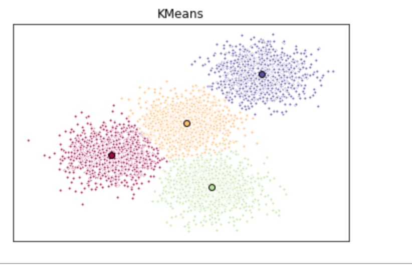
# plot the clustering result
# Initialize the plot with the specified dimensions.
fig = plt.figure(figsize=(6, 4))

# Colors uses a color map, which will produce an array of colors based on
# the number of labels there are. We use set(k_means_labels) to get the
# unique labels.
colors = plt.cm.Spectral(np.linspace(0, 1, len(set(k_means_labels))))

# Create a plot
ax = fig.add_subplot(1, 1, 1)

# For loop that plots the data points and centroids.
# k will range from 0-3, which will match the possible clusters that each
# data point is in.
for k, col in zip(range(len([[4,4], [-2, -1], [2, -3], [1, 1]])), colors):

    # Create a list of all data points, where the data poitns that are
    # in the cluster (ex. cluster 0) are labeled as true, else they are
    # labeled as false.
    my_members = (k_means_labels == k)

    # Define the centroid, or cluster center.
    cluster_center = k_means_cluster_centers[k]

    # Plots the datapoints with color col.
    ax.plot(X[my_members, 0], X[my_members, 1], 'w', markerfacecolor=col, marker='.')

    # Plots the centroids with specified color, but with a darker outline
    ax.plot(cluster_center[0], cluster_center[1], 'o', markerfacecolor=col,  markeredgecolor='k', markersize=6)

# Title of the plot
ax.set_title('KMeans')

# Remove x-axis ticks
ax.set_xticks(())

# Remove y-axis ticks
ax.set_yticks(())

# Show the plot
plt.show()

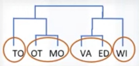
Hierarchical Clustering

Hierarchical clustering algorithms build a hierarchy of clusters where each node is a cluster consists of the clusters of its daughter nods.

Agglomerative Vs Divisive

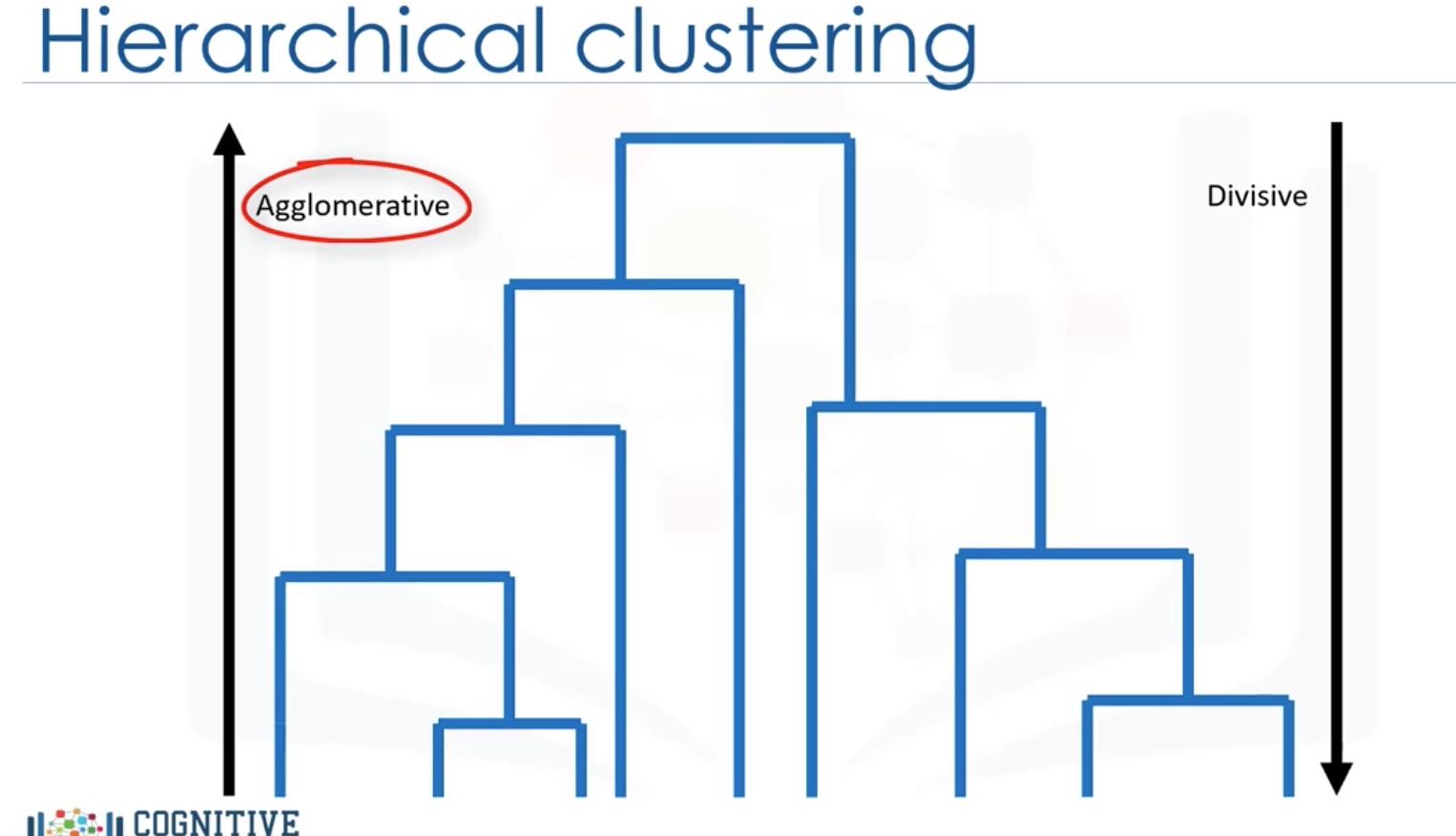
Agglomerative algorithm

• Create n clusters, one for each data point

  

• Compute the Proximity matrix

• Repeat

  • Merge the two closets clusters
  • Update the Proximity Matrix

• Until only a single cluster remains

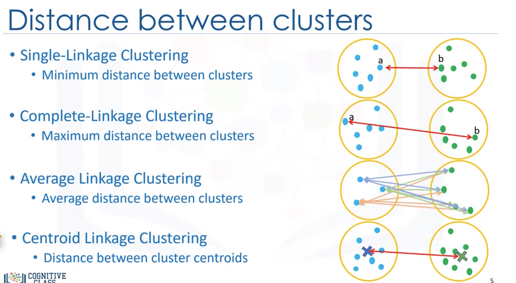
How to measure Distance between clusters:

• Single-linkage clustering: minimum distance between clusters
• Complete-linkage clustering: Maximum distance between clusters
• Average Linkage Clustering: Average distance between clusters

• Centroid Linkage clustering: distance between cluster centroids (the average of points within a cluster)

  

Advantages VS Disadvantages

K means VS Hierarchical clustering

Lab: Hierarchical Clustering

import numpy as np
import pandas as pd
from scipy import ndimage
from scipy.cluster import hierarchy
from scipy.spatial import distance_matrix
from matplotlib import pyplot as plt
from sklearn import manifold, datasets
from sklearn.cluster import AgglomerativeClustering
from sklearn.datasets.samples_generator import make_blobs
%matplotlib inline


# Generating random Data
X1, y1 = make_blobs(n_samples=50, centers=[[4,4], [-2, -1], [1, 1], [10,4]], cluster_std=0.9)

plt.scatter(X1[:, 0], X1[:, 1], marker='o')

# Agglomerative clustering
agglom = AgglomerativeClustering(n_clusters = 4, linkage = 'average')
agglom.fit(X1,y1)

# plot the clustering
# Create a figure of size 6 inches by 4 inches.
plt.figure(figsize=(6,4))

# These two lines of code are used to scale the data points down,
# Or else the data points will be scattered very far apart.

# Create a minimum and maximum range of X1.
x_min, x_max = np.min(X1, axis=0), np.max(X1, axis=0)

# Get the average distance for X1.
X1 = (X1 - x_min) / (x_max - x_min)

# This loop displays all of the datapoints.
for i in range(X1.shape[0]):
    # Replace the data points with their respective cluster value
    # (ex. 0) and is color coded with a colormap (plt.cm.spectral)
    plt.text(X1[i, 0], X1[i, 1], str(y1[i]),
            color=plt.cm.nipy_spectral(agglom.labels_[i] / 10.),
            fontdict={'weight': 'bold', 'size': 9})

# Remove the x ticks, y ticks, x and y axis
plt.xticks([])
plt.yticks([])
#plt.axis('off')



# Display the plot of the original data before clustering
plt.scatter(X1[:, 0], X1[:, 1], marker='.')
# Display the plot
plt.show()

# Dendrogram Associated for the Agglomerative Hierarchical Clustering
dist_matrix = distance_matrix(X1,X1)
print(dist_matrix)

Z = hierarchy.linkage(dist_matrix, 'complete')

dendro = hierarchy.dendrogram(Z)

Note: pd.apply()

filter(function, sequence)
# find those can be divided by 3 in range(1,11)
selected_numbers = filter(lambda x: x % 3 == 0, range(1, 11))

# apply for every element
df.apply(np.square)
# apply for specific col or row-- with the x.name or x.index to limit
df.apply(lambda x : np.square(x) if x.name=='col' else x, axis=0)
# by default axis=0, that is down the rows, and each col is applied together


df.apply(lambda x : np.square(x) if x.name=='rowname' else x, axis=1)

# convert data into numeric
# coerce: if not convertible, it will be set as np.nan
df.apply(pd.to_numeric, errors='coerce')
# ignore: keep the original value
df.apply(pd.to_numeric, errors='ignore')

# Clustering on Vehicle dataset
filename = 'cars_clus.csv'

#Read csv
pdf = pd.read_csv(filename)
print ("Shape of dataset: ", pdf.shape)

pdf.head(5)

print ("Shape of dataset before cleaning: ", pdf.size)
pdf[[ 'sales', 'resale', 'type', 'price', 'engine_s',
      'horsepow', 'wheelbas', 'width', 'length', 'curb_wgt', 'fuel_cap',
      'mpg', 'lnsales']] = pdf[['sales', 'resale', 'type', 'price', 'engine_s',
      'horsepow', 'wheelbas', 'width', 'length', 'curb_wgt', 'fuel_cap',
      'mpg', 'lnsales']].apply(pd.to_numeric, errors='coerce')
pdf = pdf.dropna()
pdf = pdf.reset_index(drop=True)
print ("Shape of dataset after cleaning: ", pdf.size)
pdf.head(5)

featureset = pdf[['engine_s',  'horsepow', 'wheelbas', 'width', 'length', 'curb_wgt', 'fuel_cap', 'mpg']]

# Normalization
from sklearn.preprocessing import MinMaxScaler
x = featureset.values #returns a numpy array
min_max_scaler = MinMaxScaler()
feature_mtx = min_max_scaler.fit_transform(x)
feature_mtx [0:5]



# clustering using scipy
import scipy
leng = feature_mtx.shape[0]
D = scipy.zeros([leng,leng])
for i in range(leng):
    for j in range(leng):
        D[i,j] = scipy.spatial.distance.euclidean(feature_mtx[i], feature_mtx[j])


import pylab
import scipy.cluster.hierarchy
Z = hierarchy.linkage(D, 'complete')

from scipy.cluster.hierarchy import fcluster
max_d = 3
clusters = fcluster(Z, max_d, criterion='distance')
clusters

from scipy.cluster.hierarchy import fcluster
k = 5
clusters = fcluster(Z, k, criterion='maxclust')
clusters

from scipy.cluster.hierarchy import fcluster
k = 5
clusters = fcluster(Z, k, criterion='maxclust')
clusters

dist_matrix = distance_matrix(feature_mtx,feature_mtx)
print(dist_matrix)


agglom = AgglomerativeClustering(n_clusters = 6, linkage = 'complete')
agglom.fit(feature_mtx)
agglom.labels_

pdf['cluster_'] = agglom.labels_
pdf.head()

import matplotlib.cm as cm
n_clusters = max(agglom.labels_)+1
colors = cm.rainbow(np.linspace(0, 1, n_clusters))
cluster_labels = list(range(0, n_clusters))

# Create a figure of size 6 inches by 4 inches.
plt.figure(figsize=(16,14))

for color, label in zip(colors, cluster_labels):
    subset = pdf[pdf.cluster_ == label]
    for i in subset.index:
            plt.text(subset.horsepow[i], subset.mpg[i],str(subset['model'][i]), rotation=25)
    plt.scatter(subset.horsepow, subset.mpg, s= subset.price*10, c=color, label='cluster'+str(label),alpha=0.5)
#    plt.scatter(subset.horsepow, subset.mpg)
plt.legend()
plt.title('Clusters')
plt.xlabel('horsepow')
plt.ylabel('mpg')


pdf.groupby(['cluster_','type'])['cluster_'].count()

agg_cars = pdf.groupby(['cluster_','type'])['horsepow','engine_s','mpg','price'].mean()
agg_cars

plt.figure(figsize=(16,10))
for color, label in zip(colors, cluster_labels):
    subset = agg_cars.loc[(label,),]
    for i in subset.index:
        plt.text(subset.loc[i][0]+5, subset.loc[i][2], 'type='+str(int(i)) + ', price='+str(int(subset.loc[i][3]))+'k')
    plt.scatter(subset.horsepow, subset.mpg, s=subset.price*20, c=color, label='cluster'+str(label))
plt.legend()
plt.title('Clusters')
plt.xlabel('horsepow')
plt.ylabel('mpg')

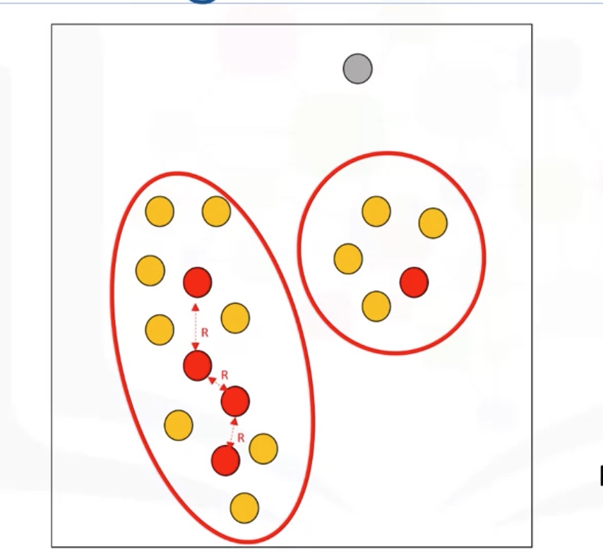
DBSCAN Clustering

DBSCAN: Density-based Spatial Clustering of Applications with noise.

• is one of the most common clustering algorithms
• works based on density of objects

R: radius of neighborhood

M: min number of neighbors

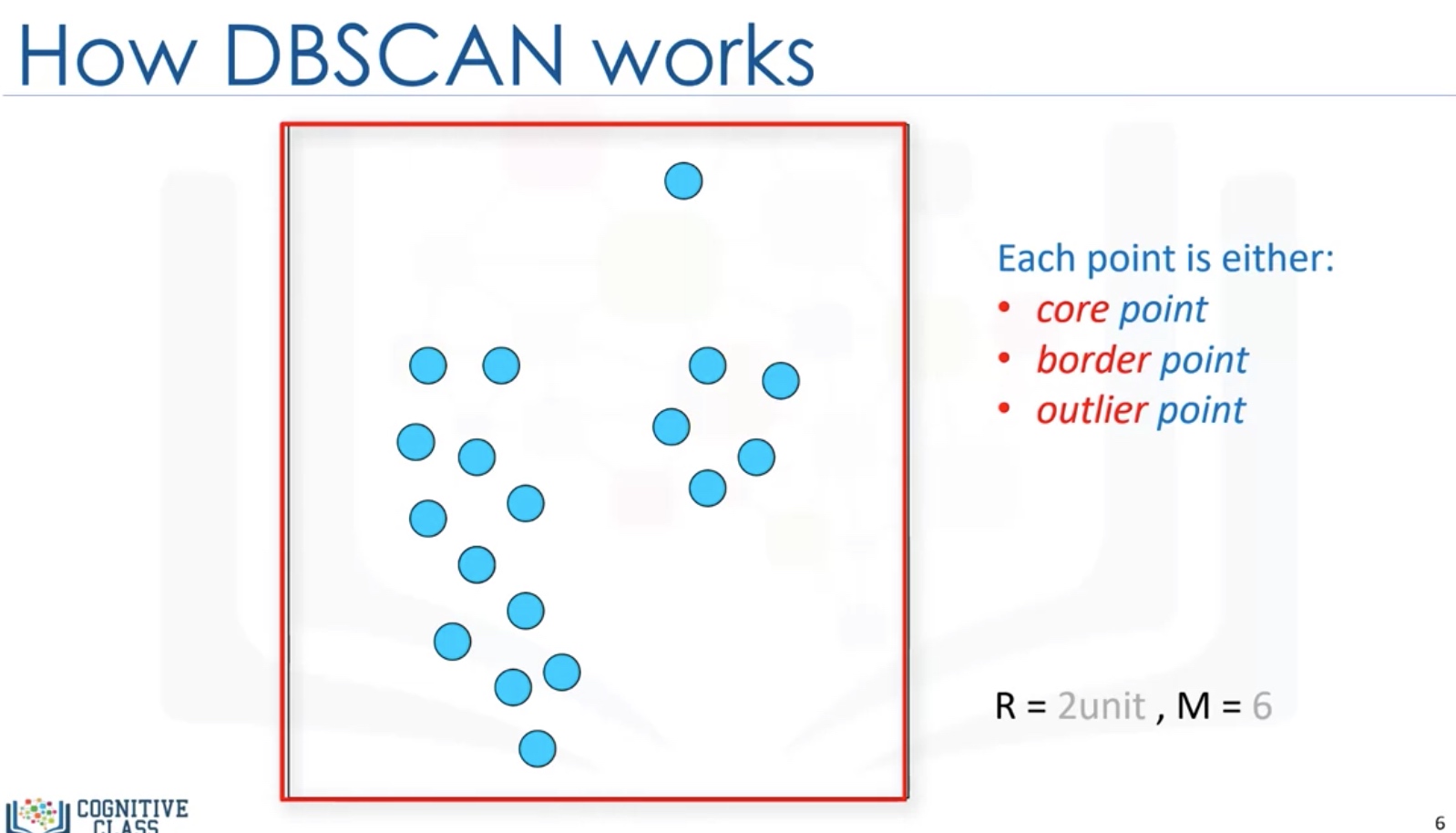
Core Point: within the radius R, there are at least M points (include the core point itself)

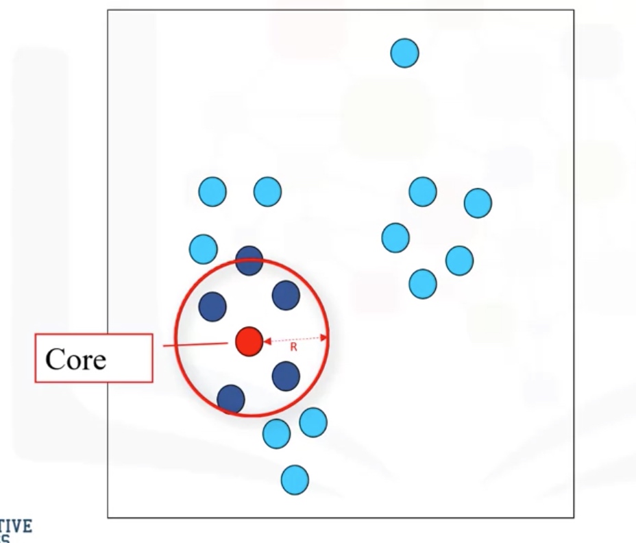
Border point: not a core point, but reachable to a core point.

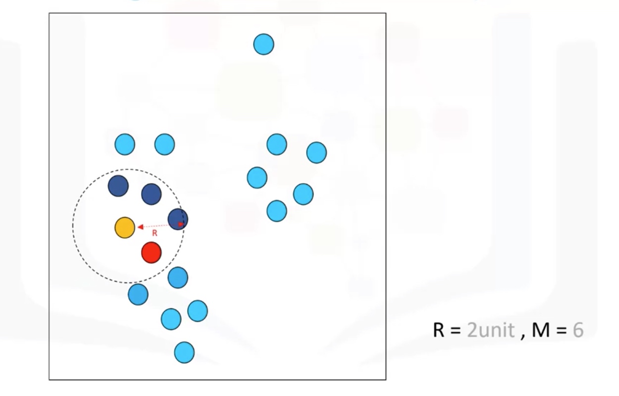
Outlier: points which cannot be reached by a core point.

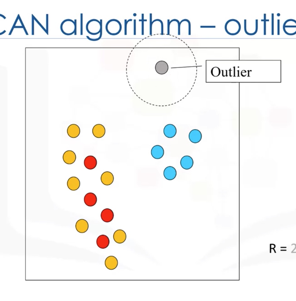
Cluster: connected core points together with their border point.

Advantages:

1. Arbitrarily shaped clusters
2. Robust to outliers
3. Does not require specification of the number of clusters

Lab: DBSCAN

import numpy as np
from sklearn.cluster import DBSCAN
from sklearn.datasets.samples_generator import make_blobs
from sklearn.preprocessing import StandardScaler
import matplotlib.pyplot as plt
%matplotlib inline


def createDataPoints(centroidLocation, numSamples, clusterDeviation):
    # Create random data and store in feature matrix X and response vector y.
    X, y = make_blobs(n_samples=numSamples, centers=centroidLocation, cluster_std=clusterDeviation)

    # Standardize features by removing the mean and scaling to unit variance
    X = StandardScaler().fit_transform(X)
    return X, y



X, y = createDataPoints([[4,3], [2,-1], [-1,4]] , 1500, 0.5)

# Training(modeling)
epsilon = 0.3
minimumSamples = 7
db = DBSCAN(eps=epsilon, min_samples=minimumSamples).fit(X)
labels = db.labels_
labels


# Distinguish outliers
# Firts, create an array of booleans using the labels from db.
core_samples_mask = np.zeros_like(db.labels_, dtype=bool)
core_samples_mask[db.core_sample_indices_] = True
core_samples_mask

# Number of clusters in labels, ignoring noise if present.
n_clusters_ = len(set(labels)) - (1 if -1 in labels else 0)
n_clusters_

# Remove repetition in labels by turning it into a set.
unique_labels = set(labels)
unique_labels

# Data Visualization
# Create colors for the clusters.
colors = plt.cm.Spectral(np.linspace(0, 1, len(unique_labels)))

# Plot the points with colors
for k, col in zip(unique_labels, colors):
    if k == -1:
        # Black used for noise.
        col = 'k'

    class_member_mask = (labels == k)

    # Plot the datapoints that are clustered
    xy = X[class_member_mask & core_samples_mask]
    plt.scatter(xy[:, 0], xy[:, 1],s=50, c=[col], marker=u'o', alpha=0.5)

    # Plot the outliers
    xy = X[class_member_mask & ~core_samples_mask]
    plt.scatter(xy[:, 0], xy[:, 1],s=50, c=[col], marker=u'o', alpha=0.5)

Real problem

!wget -O weather-stations20140101-20141231.csv https://s3-api.us-geo.objectstorage.softlayer.net/cf-courses-data/CognitiveClass/ML0101ENv3/labs/weather-stations20140101-20141231.csv

import csv
import pandas as pd
import numpy as np

filename='weather-stations20140101-20141231.csv'

#Read csv
pdf = pd.read_csv(filename)
pdf.head(5)

pdf = pdf[pd.notnull(pdf["™"])]
pdf = pdf.reset_index(drop=True)
pdf.head(5)

# Visualization
from mpl_toolkits.basemap import Basemap
import matplotlib.pyplot as plt
from pylab import rcParams
%matplotlib inline
rcParams['figure.figsize'] = (14,10)

llon=-140
ulon=-50
llat=40
ulat=65

pdf = pdf[(pdf['Long'] > llon) & (pdf['Long'] < ulon) & (pdf['Lat'] > llat) &(pdf['Lat'] < ulat)]

my_map = Basemap(projection='merc',
            resolution = 'l', area_thresh = 1000.0,
            llcrnrlon=llon, llcrnrlat=llat, #min longitude (llcrnrlon) and latitude (llcrnrlat)
            urcrnrlon=ulon, urcrnrlat=ulat) #max longitude (urcrnrlon) and latitude (urcrnrlat)

my_map.drawcoastlines()
my_map.drawcountries()
# my_map.drawmapboundary()
my_map.fillcontinents(color = 'white', alpha = 0.3)
my_map.shadedrelief()

# To collect data based on stations

xs,ys = my_map(np.asarray(pdf.Long), np.asarray(pdf.Lat))
pdf['xm']= xs.tolist()
pdf['ym'] =ys.tolist()

#Visualization1
for index,row in pdf.iterrows():
#  x,y = my_map(row.Long, row.Lat)
  my_map.plot(row.xm, row.ym,markerfacecolor =([1,0,0]),  marker='o', markersize= 5, alpha = 0.75)
#plt.text(x,y,stn)
plt.show()


# clustering of stations besed on their location
from sklearn.cluster import DBSCAN
import sklearn.utils
from sklearn.preprocessing import StandardScaler
sklearn.utils.check_random_state(1000)
Clus_dataSet = pdf[['xm','ym']]
Clus_dataSet = np.nan_to_num(Clus_dataSet)
Clus_dataSet = StandardScaler().fit_transform(Clus_dataSet)

# Compute DBSCAN
db = DBSCAN(eps=0.15, min_samples=10).fit(Clus_dataSet)
core_samples_mask = np.zeros_like(db.labels_, dtype=bool)
core_samples_mask[db.core_sample_indices_] = True
labels = db.labels_
pdf["Clus_Db"]=labels

realClusterNum=len(set(labels)) - (1 if -1 in labels else 0)
clusterNum = len(set(labels))


# A sample of clusters
pdf[["Stn_Name","Tx","™","Clus_Db"]].head(5)

set(labels)

# Visualization of clusters based on location
from mpl_toolkits.basemap import Basemap
import matplotlib.pyplot as plt
from pylab import rcParams
%matplotlib inline
rcParams['figure.figsize'] = (14,10)

my_map = Basemap(projection='merc',
            resolution = 'l', area_thresh = 1000.0,
            llcrnrlon=llon, llcrnrlat=llat, #min longitude (llcrnrlon) and latitude (llcrnrlat)
            urcrnrlon=ulon, urcrnrlat=ulat) #max longitude (urcrnrlon) and latitude (urcrnrlat)

my_map.drawcoastlines()
my_map.drawcountries()
#my_map.drawmapboundary()
my_map.fillcontinents(color = 'white', alpha = 0.3)
my_map.shadedrelief()

# To create a color map
colors = plt.get_cmap('jet')(np.linspace(0.0, 1.0, clusterNum))



#Visualization1
for clust_number in set(labels):
    c=(([0.4,0.4,0.4]) if clust_number == -1 else colors[np.int(clust_number)])
    clust_set = pdf[pdf.Clus_Db == clust_number]
    my_map.scatter(clust_set.xm, clust_set.ym, color =c,  marker='o', s= 20, alpha = 0.85)
    if clust_number != -1:
        cenx=np.mean(clust_set.xm)
        ceny=np.mean(clust_set.ym)
        plt.text(cenx,ceny,str(clust_number), fontsize=25, color='red',)
        print ("Cluster "+str(clust_number)+', Avg Temp: '+ str(np.mean(clust_set.™)))


# clustering of stations based on their location, mean ,max and min temperature
from sklearn.cluster import DBSCAN
import sklearn.utils
from sklearn.preprocessing import StandardScaler
sklearn.utils.check_random_state(1000)
Clus_dataSet = pdf[['xm','ym','Tx','™','Tn']]
Clus_dataSet = np.nan_to_num(Clus_dataSet)
Clus_dataSet = StandardScaler().fit_transform(Clus_dataSet)

# Compute DBSCAN
db = DBSCAN(eps=0.3, min_samples=10).fit(Clus_dataSet)
core_samples_mask = np.zeros_like(db.labels_, dtype=bool)
core_samples_mask[db.core_sample_indices_] = True
labels = db.labels_
pdf["Clus_Db"]=labels

realClusterNum=len(set(labels)) - (1 if -1 in labels else 0)
clusterNum = len(set(labels))


# A sample of clusters
pdf[["Stn_Name","Tx","™","Clus_Db"]].head(5)

# Visualization of clusters based on location and temperture
from mpl_toolkits.basemap import Basemap
import matplotlib.pyplot as plt
from pylab import rcParams
%matplotlib inline
rcParams['figure.figsize'] = (14,10)

my_map = Basemap(projection='merc',
            resolution = 'l', area_thresh = 1000.0,
            llcrnrlon=llon, llcrnrlat=llat, #min longitude (llcrnrlon) and latitude (llcrnrlat)
            urcrnrlon=ulon, urcrnrlat=ulat) #max longitude (urcrnrlon) and latitude (urcrnrlat)

my_map.drawcoastlines()
my_map.drawcountries()
#my_map.drawmapboundary()
my_map.fillcontinents(color = 'white', alpha = 0.3)
my_map.shadedrelief()

# To create a color map
colors = plt.get_cmap('jet')(np.linspace(0.0, 1.0, clusterNum))



#Visualization1
for clust_number in set(labels):
    c=(([0.4,0.4,0.4]) if clust_number == -1 else colors[np.int(clust_number)])
    clust_set = pdf[pdf.Clus_Db == clust_number]
    my_map.scatter(clust_set.xm, clust_set.ym, color =c,  marker='o', s= 20, alpha = 0.85)
    if clust_number != -1:
        cenx=np.mean(clust_set.xm)
        ceny=np.mean(clust_set.ym)
        plt.text(cenx,ceny,str(clust_number), fontsize=25, color='red',)
        print ("Cluster "+str(clust_number)+', Avg Temp: '+ str(np.mean(clust_set.™)))

Introduction to Recommender System

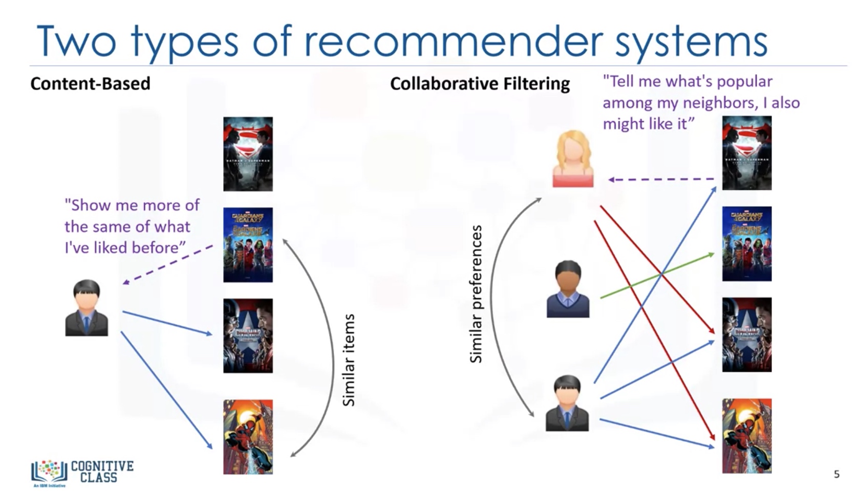
Two Types of recommender systems

Content-based: Show more of the type of content which the user has liked before. Collaborative Filtering: show more of the content which is popular among the neighbors of the client.

Implementing recommender system

• Memory-based
  • Uses the entire user-item dataset to generate a recommendation
  • uses statistical techniques to approximate users or items. E.g.: Pearson correlation, cosine similarity, euclidean distance, etc.
• Model-based
  • Develops a model of users in an attempt to learn their preference
  • Models can be created using ML techniques like regression, clustering, classification, etc.

Content-based recommender systems

In content-based recommender system, the features X of the items are available.

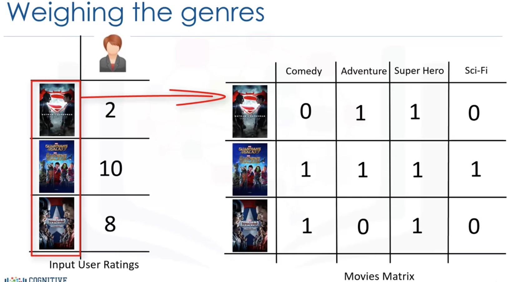
Weighing the genres

Weighted Genre Matrix = X.*r Then we can predict the user profile as the sum of each rows: (X.*r).sum(axis=0)

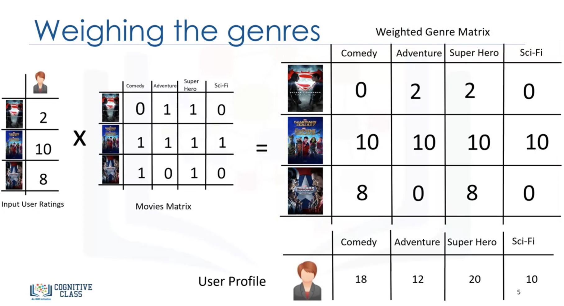
We have to normalize the user profile vector, since the it is now related to the number of ratings given by the user.

We then use the user profile vector to predict the predicted ratings: $X*\theta $

Lab: content-based recommender system

#Dataframe manipulation library
import pandas as pd
#Math functions, we'll only need the sqrt function so let's import only that
from math import sqrt
import numpy as np
import matplotlib.pyplot as plt
%matplotlib inline

#Storing the movie information into a pandas dataframe
movies_df = pd.read_csv('movies.csv')
#Storing the user information into a pandas dataframe
ratings_df = pd.read_csv('ratings.csv')
#Head is a function that gets the first N rows of a dataframe. N's default is 5.
movies_df.head()

#Using regular expressions to find a year stored between parentheses
#We specify the parantheses so we don't conflict with movies that have years in their titles
movies_df['year'] = movies_df.title.str.extract('(\(\d\d\d\d\))',expand=False)
#Removing the parentheses
movies_df['year'] = movies_df.year.str.extract('(\d\d\d\d)',expand=False)
#Removing the years from the 'title' column
movies_df['title'] = movies_df.title.str.replace('(\(\d\d\d\d\))', '')
#Applying the strip function to get rid of any ending whitespace characters that may have appeared
movies_df['title'] = movies_df['title'].apply(lambda x: x.strip())
movies_df.head()

#Every genre is separated by a | so we simply have to call the split function on |
movies_df['genres'] = movies_df.genres.str.split('|')
movies_df.head()

#Copying the movie dataframe into a new one since we won't need to use the genre information in our first case.
moviesWithGenres_df = movies_df.copy()

#For every row in the dataframe, iterate through the list of genres and place a 1 into the corresponding column
for index, row in movies_df.iterrows():
    for genre in row['genres']:
        moviesWithGenres_df.at[index, genre] = 1
#Filling in the NaN values with 0 to show that a movie doesn't have that column's genre
moviesWithGenres_df = moviesWithGenres_df.fillna(0)
moviesWithGenres_df.head()


ratings_df.head()
#Drop removes a specified row or column from a dataframe
ratings_df = ratings_df.drop('timestamp', 1)
ratings_df.head()

userInput = [
            {'title':'Breakfast Club, The', 'rating':5},
            {'title':'Toy Story', 'rating':3.5},
            {'title':'Jumanji', 'rating':2},
            {'title':"Pulp Fiction", 'rating':5},
            {'title':'Akira', 'rating':4.5}
        ]
inputMovies = pd.DataFrame(userInput)
inputMovies

# Add movieID to input user
#Filtering out the movies by title
inputId = movies_df[movies_df['title'].isin(inputMovies['title'].tolist())]
#Then merging it so we can get the movieId. It's implicitly merging it by title.
inputMovies = pd.merge(inputId, inputMovies)
#Dropping information we won't use from the input dataframe
inputMovies = inputMovies.drop('genres', 1).drop('year', 1)
#Final input dataframe
#If a movie you added in above isn't here, then it might not be in the original
#dataframe or it might spelled differently, please check capitalisation.
inputMovies


#Filtering out the movies from the input
userMovies = moviesWithGenres_df[moviesWithGenres_df['movieId'].isin(inputMovies['movieId'].tolist())]
userMovies

#Resetting the index to avoid future issues
userMovies = userMovies.reset_index(drop=True)
#Dropping unnecessary issues due to save memory and to avoid issues
userGenreTable = userMovies.drop('movieId', 1).drop('title', 1).drop('genres', 1).drop('year', 1)
userGenreTable

inputMovies['rating']

#Dot produt to get weights
userProfile = userGenreTable.transpose().dot(inputMovies['rating'])
#The user profile
userProfile

#Now let's get the genres of every movie in our original dataframe
genreTable = moviesWithGenres_df.set_index(moviesWithGenres_df['movieId'])
#And drop the unnecessary information
genreTable = genreTable.drop('movieId', 1).drop('title', 1).drop('genres', 1).drop('year', 1)
genreTable.head()

#Multiply the genres by the weights and then take the weighted average
recommendationTable_df = ((genreTable*userProfile).sum(axis=1))/(userProfile.sum())
recommendationTable_df.head()

#Sort our recommendations in descending order
recommendationTable_df = recommendationTable_df.sort_values(ascending=False)
#Just a peek at the values
recommendationTable_df.head()

#The final recommendation table
movies_df.loc[movies_df['movieId'].isin(recommendationTable_df.head(20).keys())]

Collaborative Filtering

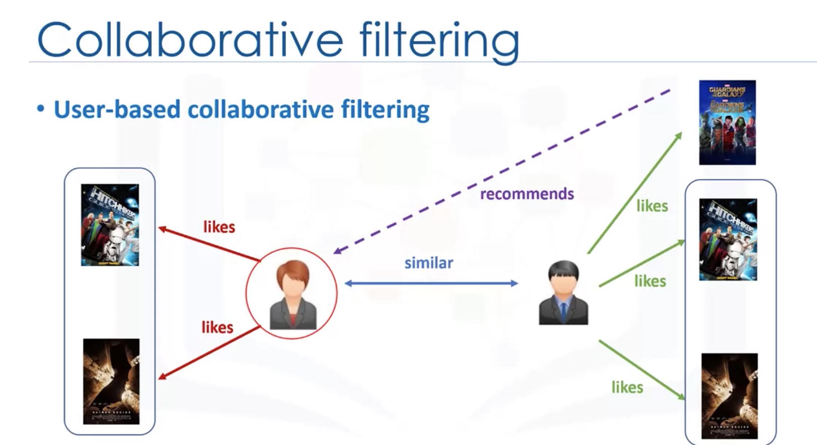
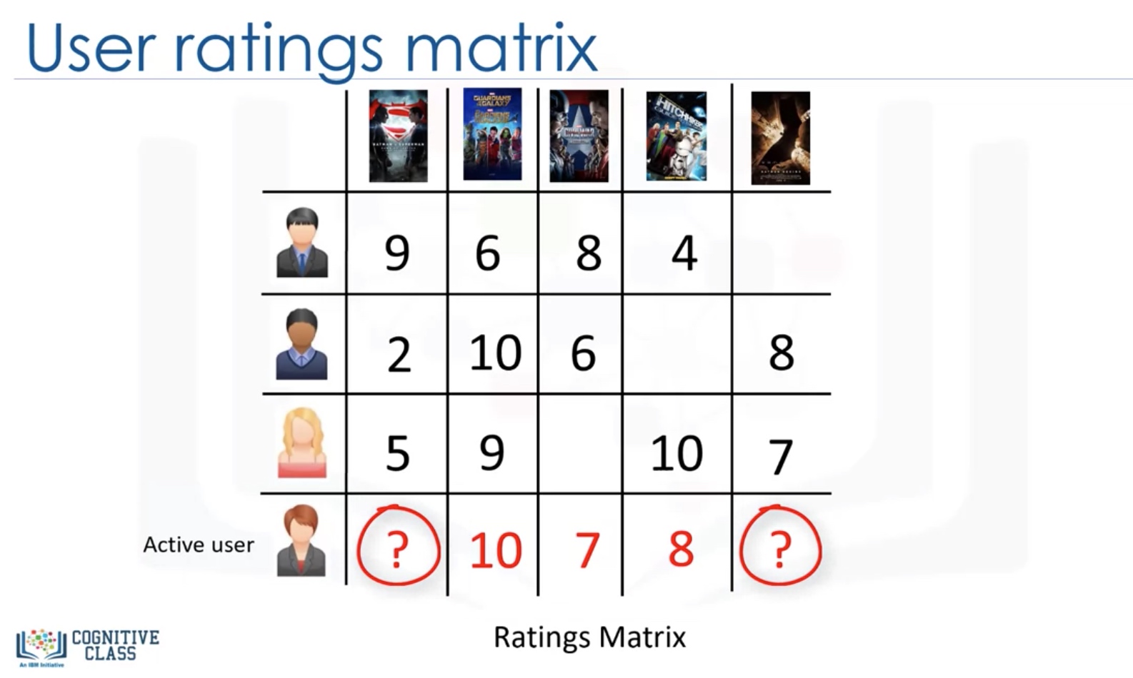
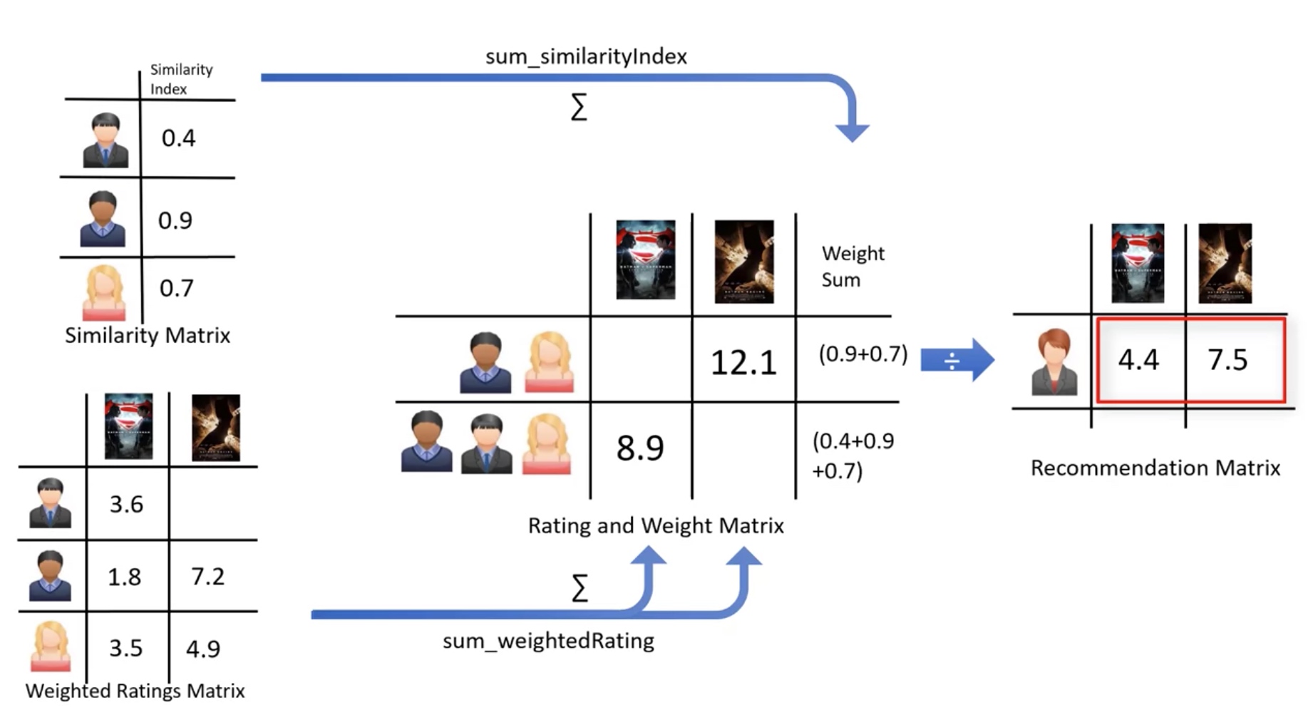
User-based VS Item-based

Challenges of collaborative filtering

• Data Sparcity
  • Users in general rate only a limited number of items
• Cold start
  • Difficulty in recommendations to new users or new items
• Scalibility
  • Increase in number of users or items

Lab: Collaborative filtering on movies

# Preprocessing
#Dataframe manipulation library
import pandas as pd
#Math functions, we'll only need the sqrt function so let's import only that
from math import sqrt
import numpy as np
import matplotlib.pyplot as plt
%matplotlib inline

#Storing the movie information into a pandas dataframe
movies_df = pd.read_csv('movies.csv')
#Storing the user information into a pandas dataframe
ratings_df = pd.read_csv('ratings.csv')

#Head is a function that gets the first N rows of a dataframe. N's default is 5.
movies_df.head()

#Using regular expressions to find a year stored between parentheses
#We specify the parantheses so we don't conflict with movies that have years in their titles
movies_df['year'] = movies_df.title.str.extract('(\(\d\d\d\d\))',expand=False)
#Removing the parentheses
movies_df['year'] = movies_df.year.str.extract('(\d\d\d\d)',expand=False)
#Removing the years from the 'title' column
movies_df['title'] = movies_df.title.str.replace('(\(\d\d\d\d\))', '')
#Applying the strip function to get rid of any ending whitespace characters that may have appeared
movies_df['title'] = movies_df['title'].apply(lambda x: x.strip())


#Dropping the genres column
movies_df = movies_df.drop('genres', 1)

#Drop removes a specified row or column from a dataframe
ratings_df = ratings_df.drop('timestamp', 1)

# Collaborative filtering

userInput = [
            {'title':'Breakfast Club, The', 'rating':5},
            {'title':'Toy Story', 'rating':3.5},
            {'title':'Jumanji', 'rating':2},
            {'title':"Pulp Fiction", 'rating':5},
            {'title':'Akira', 'rating':4.5}
        ]
inputMovies = pd.DataFrame(userInput)
inputMovies


#Filtering out the movies by title
inputId = movies_df[movies_df['title'].isin(inputMovies['title'].tolist())]
#Then merging it so we can get the movieId. It's implicitly merging it by title.
inputMovies = pd.merge(inputId, inputMovies)
#Dropping information we won't use from the input dataframe
inputMovies = inputMovies.drop('year', 1)
#Final input dataframe
#If a movie you added in above isn't here, then it might not be in the original
#dataframe or it might spelled differently, please check capitalisation.
inputMovies

#Filtering out users that have watched movies that the input has watched and storing it
userSubset = ratings_df[ratings_df['movieId'].isin(inputMovies['movieId'].tolist())]
userSubset.head()

#Groupby creates several sub dataframes where they all have the same value in the column specified as the parameter
userSubsetGroup = userSubset.groupby(['userId'])

# Lets look at the one of the users: ID=1130
userSubsetGroup.get_group(1130)

#Sorting it so users with movie most in common with the input will have priority
userSubsetGroup = sorted(userSubsetGroup,  key=lambda x: len(x[1]), reverse=True)

# We will select a subset of users to iterate through. This limit is imposed because we don't want to waste too much time going through every single user.

userSubsetGroup = userSubsetGroup[0:100]

#Store the Pearson Correlation in a dictionary, where the key is the user Id and the value is the coefficient
pearsonCorrelationDict = {}

#For every user group in our subset
for name, group in userSubsetGroup:
    #Let's start by sorting the input and current user group so the values aren't mixed up later on
    group = group.sort_values(by='movieId')
    inputMovies = inputMovies.sort_values(by='movieId')
    #Get the N for the formula
    nRatings = len(group)
    #Get the review scores for the movies that they both have in common
    temp_df = inputMovies[inputMovies['movieId'].isin(group['movieId'].tolist())]
    #And then store them in a temporary buffer variable in a list format to facilitate future calculations
    tempRatingList = temp_df['rating'].tolist()
    #Let's also put the current user group reviews in a list format
    tempGroupList = group['rating'].tolist()
    #Now let's calculate the pearson correlation between two users, so called, x and y
    Sxx = sum([i**2 for i in tempRatingList]) - pow(sum(tempRatingList),2)/float(nRatings)
    Syy = sum([i**2 for i in tempGroupList]) - pow(sum(tempGroupList),2)/float(nRatings)
    Sxy = sum( i*j for i, j in zip(tempRatingList, tempGroupList)) - sum(tempRatingList)*sum(tempGroupList)/float(nRatings)

    #If the denominator is different than zero, then divide, else, 0 correlation.
    if Sxx != 0 and Syy != 0:
        pearsonCorrelationDict[name] = Sxy/sqrt(Sxx*Syy)
    else:
        pearsonCorrelationDict[name] = 0


pearsonCorrelationDict.items()

pearsonDF = pd.DataFrame.from_dict(pearsonCorrelationDict, orient='index')
pearsonDF.columns = ['similarityIndex']
pearsonDF['userId'] = pearsonDF.index
pearsonDF.index = range(len(pearsonDF))
pearsonDF.head()


topUsers=pearsonDF.sort_values(by='similarityIndex', ascending=False)[0:50]
topUsers.head()


topUsersRating=topUsers.merge(ratings_df, left_on='userId', right_on='userId', how='inner')
topUsersRating.head()

#Multiplies the similarity by the user's ratings
topUsersRating['weightedRating'] = topUsersRating['similarityIndex']*topUsersRating['rating']
topUsersRating.head()

#Applies a sum to the topUsers after grouping it up by userId
tempTopUsersRating = topUsersRating.groupby('movieId').sum()[['similarityIndex','weightedRating']]
tempTopUsersRating.columns = ['sum_similarityIndex','sum_weightedRating']
tempTopUsersRating.head()


#Creates an empty dataframe
recommendation_df = pd.DataFrame()
#Now we take the weighted average
recommendation_df['weighted average recommendation score'] = tempTopUsersRating['sum_weightedRating']/tempTopUsersRating['sum_similarityIndex']
recommendation_df['movieId'] = tempTopUsersRating.index
recommendation_df.head()

recommendation_df = recommendation_df.sort_values(by='weighted average recommendation score', ascending=False)
recommendation_df.head(10)

movies_df.loc[movies_df['movieId'].isin(recommendation_df.head(10)['movieId'].tolist())]

Final Assignment

import itertools
import numpy as np
import matplotlib.pyplot as plt
from matplotlib.ticker import NullFormatter
import pandas as pd
import numpy as np
import matplotlib.ticker as ticker
from sklearn import preprocessing
%matplotlib inline

df = pd.read_csv('loan_train.csv')
df.head()

df['due_date'] = pd.to_datetime(df['due_date'])
df['effective_date'] = pd.to_datetime(df['effective_date'])
df.head()

df['loan_status'].value_counts()


# sns.FacetGrid
# on principle
import seaborn as sns

bins = np.linspace(df.Principal.min(), df.Principal.max(), 10)
g = sns.FacetGrid(df, col="Gender", hue="loan_status", palette="Set1", col_wrap=2)
g.map(plt.hist, 'Principal', bins=bins, ec="k")

g.axes[-1].legend()
plt.show()

# on payment status
bins = np.linspace(df.age.min(), df.age.max(), 10)
g = sns.FacetGrid(df, col="Gender", hue="loan_status", palette="Set1", col_wrap=2)
g.map(plt.hist, 'age', bins=bins, ec="k")

g.axes[-1].legend()
plt.show()

# day of week
df['dayofweek'] = df['effective_date'].dt.dayofweek
bins = np.linspace(df.dayofweek.min(), df.dayofweek.max(), 10)
g = sns.FacetGrid(df, col="Gender", hue="loan_status", palette="Set1", col_wrap=2)
g.map(plt.hist, 'dayofweek', bins=bins, ec="k")
g.axes[-1].legend()
plt.show()


# feature binarization
df['weekend'] = df['dayofweek'].apply(lambda x: 1 if (x>3)  else 0)
df.head()

# Convert Categorical Features to numerical values
df.groupby(['Gender'])['loan_status'].value_counts(normalize=True)

# Here normalize=True will give the probability instead of the number.

df['Gender'].replace(to_replace=['male','female'], value=[0,1],inplace=True)
df.head()


df.groupby(['education'])['loan_status'].value_counts(normalize=True)

# How about education
df.groupby(['education'])['loan_status'].value_counts(normalize=True)

# Use one hot encoding technique to conver categorical varables to binary variables and append them to the feature Data Frame

Feature = df[['Principal','terms','age','Gender','weekend']]
Feature = pd.concat([Feature,pd.get_dummies(df['education'])], axis=1)
Feature.drop(['Master or Above'], axis = 1,inplace=True)
Feature.head()

# Feature selection
X = Feature
X[0:5]

y = df['loan_status'].values
y[0:5]

# Normalize Data
X= preprocessing.StandardScaler().fit(X).transform(X)
X[0:5]

# Classification
# KNN
# Train Test Split
from sklearn.model_selection import train_test_split
X_train, X_test, y_train, y_test = train_test_split( X, y, test_size=0.3, random_state=4)
print ('Train set:', X_train.shape,  y_train.shape)
print ('Test set:', X_test.shape,  y_test.shape)

# Find the Best K
from sklearn.neighbors import KNeighborsClassifier
from sklearn import metrics

Ks = 10
mean_acc = np.zeros((Ks-1))
std_acc = np.zeros((Ks-1))
ConfustionMx = [];
for n in range(1,Ks):

    #Train Model and Predict
    neigh = KNeighborsClassifier(n_neighbors = n).fit(X_train,y_train)
    yhat=neigh.predict(X_test)
    mean_acc[n-1] = metrics.accuracy_score(y_test, yhat)


    std_acc[n-1]=np.std(yhat==y_test)/np.sqrt(yhat.shape[0])

mean_acc

plt.plot(range(1,Ks),mean_acc,'g')
plt.fill_between(range(1,Ks),mean_acc - 3 * std_acc,mean_acc + 3 * std_acc, alpha=0.10)
plt.legend(('Accuracy ', '+/- 3xstd'))
plt.ylabel('Accuracy ')
plt.xlabel('Number of Nabors (K)')
plt.tight_layout()
plt.show()

# Train with the Best K
# Train data
k = 5
#Train Model and Predict
neigh = KNeighborsClassifier(n_neighbors = k).fit(X,y)
neigh
yhat_KNN = neigh.predict(X)

# Evaluation
from sklearn import metrics
print("Train set Accuracy: ", metrics.accuracy_score(y, neigh.predict(X)))

# Decision Tree
from sklearn.tree import DecisionTreeClassifier
from sklearn.model_selection import train_test_split
# X_trainset, X_testset, y_trainset, y_testset = train_test_split(X, y, test_size=0.3, random_state=3)

# Train the model
drugTree = DecisionTreeClassifier(criterion="entropy", max_depth = 6)
drugTree # it shows the default parameters

drugTree.fit(X,y)

yhat_predTree = drugTree.predict(X)

#SVM
# Training/Modeling
from sklearn import svm
clf = svm.SVC(kernel='rbf')
clf.fit(X, y)

yhat_svm = clf.predict(X)
yhat [0:5]

# Logistic Regression

# Split the test and train set
from sklearn.model_selection import train_test_split

# Training
from sklearn.linear_model import LogisticRegression
from sklearn.metrics import confusion_matrix
LR = LogisticRegression(C=0.01, solver='liblinear').fit(X,y)
LR

yhat_lr = LR.predict(X)
yhat_lr


# Evaluation
from sklearn.metrics import jaccard_similarity_score
from sklearn.metrics import f1_score
from sklearn.metrics import log_loss

# Load test set for evaluation
test_df = pd.read_csv('loan_test.csv')
test_df.head()
test_df['due_date'] = pd.to_datetime(test_df['due_date'])
test_df['effective_date'] = pd.to_datetime(test_df['effective_date'])
test_df.head()

test_df['dayofweek'] = test_df['effective_date'].dt.dayofweek
test_df['weekend'] = test_df['dayofweek'].apply(lambda x: 1 if (x>3)  else 0)
test_df.head()

test_df.groupby(['Gender'])['loan_status'].value_counts(normalize=True)

test_df['Gender'].replace(to_replace=['male','female'], value=[0,1],inplace=True)
test_df.head()


test_df.groupby(['education'])['loan_status'].value_counts(normalize=True)

Feature_test = test_df[['Principal','terms','age','Gender','weekend']]
Feature_test = pd.concat([Feature_test,pd.get_dummies(test_df['education'])], axis=1)
Feature_test.drop(['Master or Above'], axis = 1,inplace=True)
Feature_test.head()

X_test = Feature_test
X_test[0:5]

y_test = test_df['loan_status'].values
y_test[0:5]

X_test= preprocessing.StandardScaler().fit(X_test).transform(X_test)
X_test[0:5]

yh_knn=neigh.predict(X_test)
yh_dt=drugTree.predict(X_test)
yh_svm = clf.predict(X_test)
yh_lr=LR.predict(X_test)

yhat_all=[yh_knn,yh_dt,yh_svm,yh_lr]

# Report
# f1_score
score_f1=[]
for yi in yhat_all:
    score_f1.append(f1_score(y_test, yi, average='weighted') )


#jaccard_similarity_score
score_jaccard=[]
for yi in yhat_all:
    score_jaccard.append(jaccard_similarity_score(y_test, yi) )


#log loss

# y_test_num=pd.DataFrame(y_test).iloc[:,0].apply(lambda x:1  if (x=="PAIDOFF") else 0 ).tolist()
# yh_lr_num=pd.DataFrame(yh_lr).iloc[:,0].apply(lambda x:1  if (x=="PAIDOFF") else 0 ).tolist()
yh_lr_prob = LR.predict_proba(X_test)
# use the predicted probability to calculate the log_loss
score_logloss=log_loss(y_test, yh_lr_prob)
score_logloss=np.array([np.nan,np.nan,np.nan,score_logloss])

# Final report
df_result=pd.DataFrame(index=['KNN','Decision Tree','SVM','LogisticRegression'],columns=['Jaccard','F1-score','LogLoss'])
df_result.index.name='Algorithm'
df_result.Jaccard=score_jaccard
df_result.iloc[:,1]=score_f1
df_result.iloc[:,2]=score_logloss
df_result