Chapter 1: Some Basic Math
Log return and standard return
One of the most common applications of logarithms in finance is computing log returns. Log returns are defined as follows:
\[\begin{equation} r_{t} \equiv \ln \left(1+R_{t}\right) \quad \text { where } \quad R_{t}=\frac{P_{t}-P_{t-1}}{P_{t-1}} \end{equation}\]Alternatively:
\[e^{r_t}= 1+R_{t}=\frac{P_{t}}{P_{t-1}}\]To get a more precise estimate of the relationship between standard returns and log returns, we can use the following approximation:
\[r\approx R-\frac{1}{2}R^2\]Compounding
To get the return of a security for two periods using simple returns, we have to do something that is not very intuitive, namely adding one to each of the returns, multiplying, and then subtracting one:
\[\begin{equation} R_{2, t}=\frac{P_{t}-P_{t-2}}{P_{t-2}}=\left(1+R_{1, t}\right)\left(1+R_{1, t-1}\right)-1 \end{equation}\]and for the log return:
\[r_{2,t}=r_{1,t}+r_{1,t-1}\]Log return and log price
Define $p_t$ as the log of price $P_t$, then we have:
\[r_t=ln(P_t/P_{t-1})=p_t-p_{t-1}\]As a result, we can check the log(price)-Time plot, to see whether the return is increasing:

According to the graph above, the log return is constant, even though the price is increasing faster than a linear speed.
Chapter 2: Basic Statistics
Population and Sample Data
The state of absolute certainty is, unfortunately, quite rare in finance. More often, we are faced with a situation such as this: estimate the mean return of stock ABC, given the most recent year of daily returns. In a situation like this, we assume there is some underlying data-generating process, whose statistical properties are constant over time.
We can only estimate the true mean based on our limited data sample. In our example, assuming n returns, we estimate the mean using the same formula as before:
\[\begin{equation} \hat{\mu}=\frac{1}{n} \sum_{i=1}^{n} r_{i}=\frac{1}{n}\left(r_{1}+r_{2}+\cdots+r_{n-1}+r_{n}\right) \end{equation}\]where $\hat{\mu}$ (pronounced “mu hat”) is our estimate of the true mean, μ, based on our sample of n returns. We call this the sample mean.
Variance and Standard Deviation
The variance of a random variable measures how noisy or unpredictable that random variable is. Variance is defined as the expected value of the difference between the variable and its mean squared:
\[\sigma^2=E[(X-\mu)^2 ]\]The square root of variance, typically denoted by σ , is called standard deviation. In finance we often refer to standard deviation as volatility. This is analogous to referring to the mean as the average. Standard deviation is a mathematically precise term, whereas volatility is a more general concept.
In the previous example, we were calculating the population variance and standard deviation. All of the possible outcomes for the derivative were known.
To calculate the sample variance of a random variable X based on n observations, $x_1,x_2,…,x_n$ and the sample mean $\hat{\mu}$, we can use the following formula:
\[\begin{equation} \begin{array}{l} \hat{\sigma}_{x}^{2}=\frac{1}{n-1} \sum_{i=1}^{n}\left(x_{i}-\hat{\mu}_{x}\right)^2 \\ E\left[\hat{\sigma}_{x}^{2}\right]=\sigma_{x}^{2} \end{array} \end{equation}\]We divide the sum of squared errors by n-1 to arrive at a unbiased estimator of true variance. If the mean is known or we are calculating the population variance, then we divide by n. If instead the mean is also being estimated, then we divide by n − 1.
It can easily be rearranged as follows:
\[\sigma^{2}=E\left[X^{2}\right]-\mu^{2}=E\left[X^{2}\right]-E[X]^{2}\]Covariance and Correlation
Covariance is analogous to variance, but instead of looking at the deviation from the mean of one variable, we are going to look at the relationship between the deviations of two variables:
\[\sigma_{X Y}=E\left[\left(X-\mu_{X}\right)\left(Y-\mu_{Y}\right)\right]\]Just as we rewrote our variance equation earlier, we can rewrite the previous equation as follows:
\[\sigma_{X Y}=E\left[\left(X-\mu_{X}\right)\left(Y-\mu_{Y}\right)\right]=E[X Y]-\mu_{X} \mu_{Y}=E[X Y]-E[X] E[Y]\]In order to calculate the covariance between two random variables, X and Y, assuming the means of both variables are known, we can use the following formula:
\[\hat{\sigma}_{X, Y}=\frac{1}{n} \sum_{i=1}^{n}\left(x_{i}-\mu_{X}\right)\left(y_{i}-\mu_{Y}\right)\]If the means are unknown and must also be estimated, we replace n with (n − 1):
\[\hat{\sigma}_{X, Y}=\frac{1}{n-1} \sum_{i=1}^{n}\left(x_{i}-\hat{\mu_{X}}\right)\left(y_{i}-\hat{\mu_{Y}}\right)\]To get rid of the the impact of each variable’s deviation on the covariance, we can use the correlation:
\[\rho_{XY}=\frac{\sigma_{XY}}{\sigma_X \sigma_Y}\]If two variables are highly correlated, it is often the case that one variable causes the other variable, or that both variables share a common underlying driver.
However, Correlation does not prove causation. Similarly, if two variables are uncorrelated, it does not necessarily follow that they are unrelated.
For example, assume X is a random variable, and Y = $X^2$. X has an equal probability of being −1, 0, or +1. The correlation between X and Y is 0.
Application: Portfolio Variance and Hedging
For example, if we have two securities with random returns $X_A$ and $X_B$, with means $\mu_A$ and $\mu_B$ and standard deviations $\sigma_A$ and $\sigma_B$, respectively, we can calculate the variance of $X_A+X_B$ as follows:
\[\sigma^2_{A+B}=\sigma^2_{A}+\sigma^2_{B}+2\rho_{AB}\sigma_A \sigma_B\]Since we know that the $\rho \in [-1,1]$, the portfolio has a minimum of variance if $\rho = -1$.
If the variance of both securities is equal, then Equation simplifies to:
\[\sigma^2_{A+B}=2 \sigma^2 (1+\rho_{AB})\]In the special case where the correlation between the two securities is zero, we can further simplify our equation. For the standard deviation
\[\rho_{AB}=0 \Longrightarrow \sigma_{A+B}=\sqrt{2} \sigma\]If Y is a linear combination of $X_A$ and $X_B$, such that:
\[Y=aX_A+bX_B\]then, using our standard notation, we have:
\[\sigma^2_Y=a^2 \sigma^2_A +b^2 \sigma^2_B + 2ab \rho_{AB}\sigma_A \sigma_B\]Correlation is central to the problem of hedging. Using the same notation as before, imagine we have 1 dollar of Security A, and we wish to hedge it with h dollar of Security B.
\[\begin{aligned} P &=X_{A}+h X_{B} \\ \sigma_{P}^{2} &=\sigma_{A}^{2}+h^{2} \sigma_{B}^{2}+2 h \rho_{A B} \sigma_{A} \sigma_{B} \end{aligned}\]As a risk manager, we might be interested to know what hedge ratio would achieve the portfolio with the least variance:
\[\begin{aligned} \frac{d \sigma_{P}^{2}}{d h} &=2 h \sigma_{B}^{2}+2 \rho_{A B} \sigma_{A} \sigma_{B} \\ h^{*} &=-\rho_{A B} \frac{\sigma_{A}}{\sigma_{B}} \end{aligned}\]Substituting $h^*$ back into our original equation, we see that the smallest variance we can achieve is:
\[\min \left[\sigma_{P}^{2}\right]=\sigma_{A}^{2}\left(1-\rho_{A B}^{2}\right)\]This risk that we cannot hedge is referred to as idiosyncratic risk.
Moments
Previously, we defined the mean of a variable X as:
\[\mu = E[X]\]It turns out that we can generalize this concept as follows:
\[m_k= E[X^k]\]We refer to $m_k$ as the k-th moment of X. The mean of X is also the first moment of X.
Similarly, we can generalize the concept of variance as follows:
\[\mu_k = E[(X-\mu)^k]\]We refer to $μ_k$ as the kth central moment of X.
While we can easily calculate any central moment, in risk management it is very rare that we are interested in anything beyond the fourth central moment.
Skewness
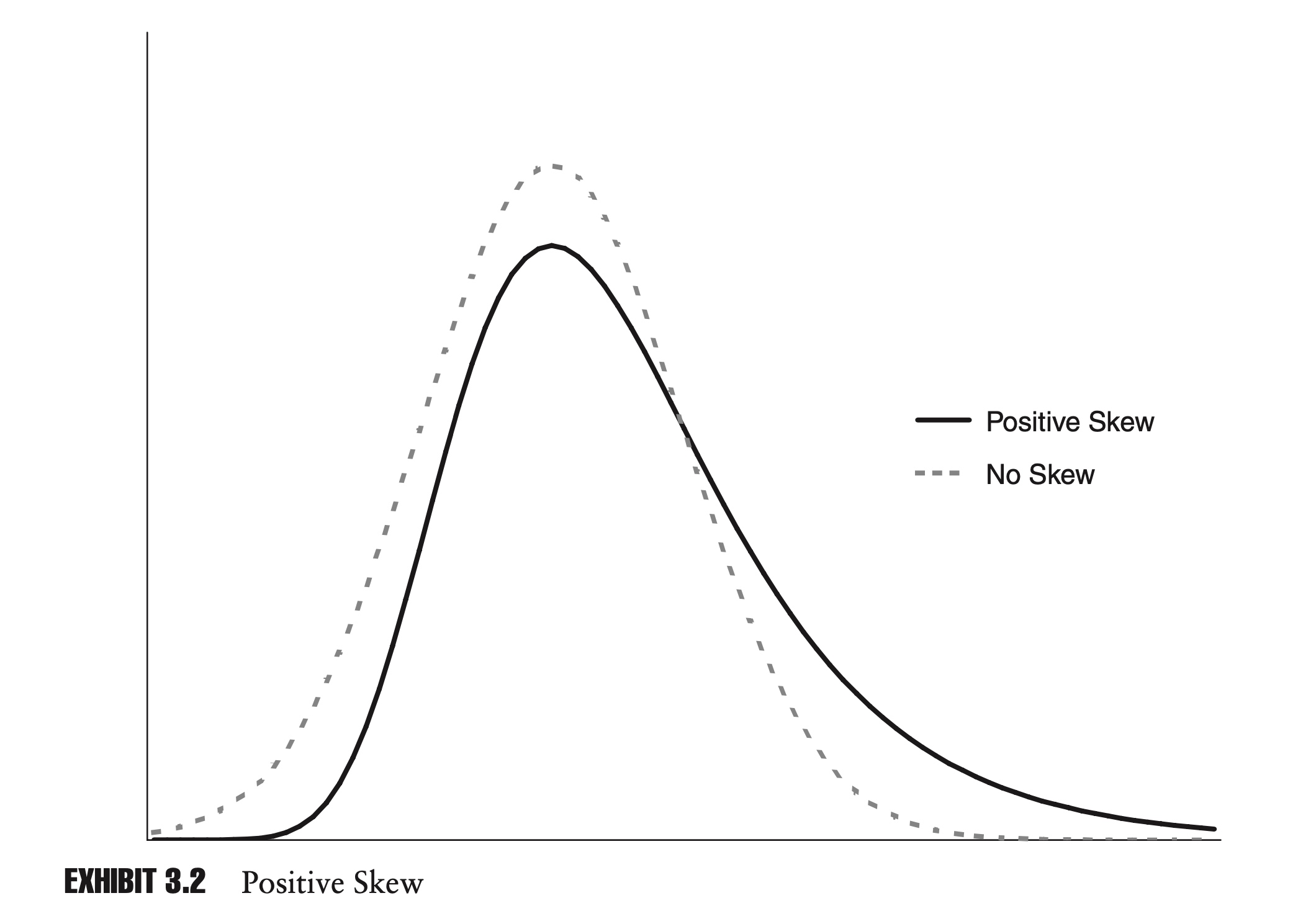
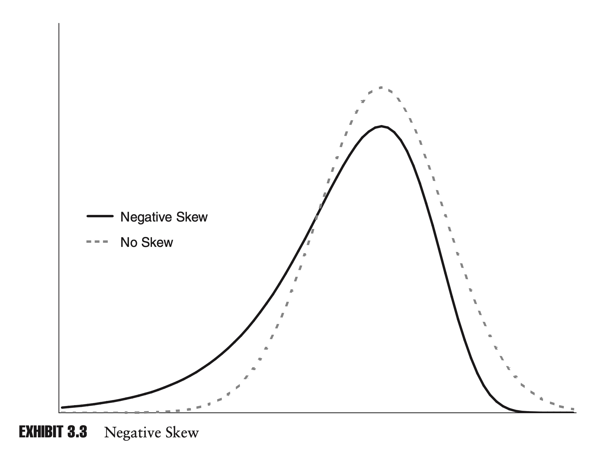
The third central moment tells us how symmetrical the distribution is around the mean. Rather than working with the third central moment directly, by convention we first standardize the statistic. The standardized third central moment is known as skewness:
\[\text{Skewness} = \frac{E[(x-\mu)^3]}{\sigma^3}\]Skewness is a very important concept in risk management. If the distributions of returns of two investments are the same in all respects, with the same mean and standard deviation, but different skews, then the investment with more negative skew is generally considered to be more risky. Historical data suggest that many financial assets exhibit negative skew.
With the population statistic, the skewness of a random variable X, based on n observations, $x_1, x_2,…, x_n$, can be calculated as:
\[\hat{s}=\frac{1}{n} \sum_{i=1}^{n}\left(\frac{x_{i}-\mu}{\sigma}\right)^{3}\]where μ is the population mean and σ is the population standard deviation.
Similar to our calculation of sample variance, if we are calculating the sample skewness there is going to be an overlap with the calculation of the sample mean and sample standard deviation. We need to correct for that. The sample skewness can be calculated as:
\[\tilde{s}=\frac{n}{(n-1)(n-2)} \sum_{i=1}^{n}\left(\frac{x_{i}-\hat{\mu}}{\hat{\sigma}}\right)^{3}\]We also have:
\[E[(X-\mu)^3]=E[X^3]-3\mu \sigma^2 -\mu^3\]Kurtosis
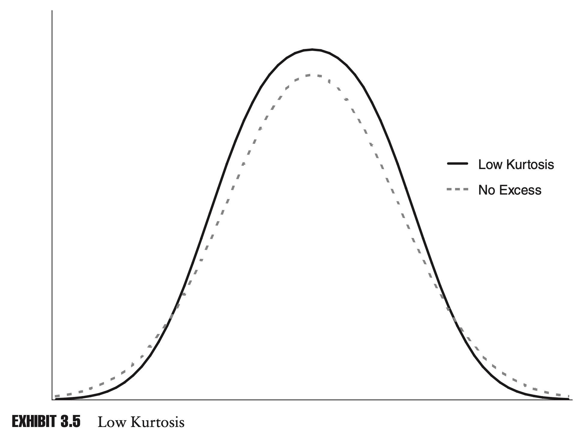
The fourth central moment is similar to the second central moment, in that it tells us how spread out a random variable is, but it puts more weight on extreme points.
As with skewness, rather than working with the central moment directly, we typically work with a standardized statistic. This standardized fourth central moment is known as kurtosis. For a random variable X, we can define the kurtosis as K, where:
\[K=\frac{E[(X-\mu)^4]}{\sigma^4}\]Because the random variable with higher kurtosis has points further from the mean, we often refer to distribution with high kurtosis as fat-tailed.

Like skewness, kurtosis is an important concept in risk management. Many financial assets exhibit high levels of kurtosis.
If the distribution of returns of two assets have the same mean, variance, and skewness but different kurtosis, then the distribution with the higher kurtosis will tend to have more extreme points, and be considered more risky.
With the population statistic, the kurtosis of a random variable X, based on n observations, $x_1, x_2,…, x_n$, can be calculated as:
\[\hat{K}=\frac{1}{n} \sum_{i=1}^{n}\left(\frac{x_{i}-\mu}{\sigma}\right)^{4}\]where μ is the population mean and σ is the population standard deviation.
Similar to our calculation of sample variance, if we are calculating the sample kurtosis there is going to be an overlap with the calculation of the sample mean and sample standard deviation. We need to correct for that. The sample kurtosis can be calculated as:
\[\tilde{K}=\frac{n(n+1)}{(n-1)(n-2)(n-3)} \sum_{i=1}^{n}\left(\frac{x_{i}-\hat{\mu}}{\hat{\sigma}}\right)^{4}\]The normal distribution has a kurtosis of 3. Because normal distributions are so common, many people refer to “excess kurtosis”, which is simply the kurtosis minus 3.
\[K_{excess}=K-3\]When we are also using the sample mean and variance, calculating the sample excess kurtosis is somewhat more complicated than just subtracting 3. If we have n points, then the correct formula is
\[\tilde{K}_{\mathrm{excess}}=\tilde{K}-3 \frac{(n-1)^{2}}{(n-2)(n-3)}\]Best Linear Unbiased Estimator (BLUE)
In this chapter we have been careful to differentiate between the true parameters of a distribution and estimates of those parameters based on a sample of population data. In statistics we refer to these parameter estimates, or to the method of obtaining the estimate, as an estimator.
For example, at the start of the chapter, we intro- duced an estimator for the sample mean:
\[\hat{\mu}=\frac{1}{n}\sum_{i=1}^n x_i\]One justification that we gave earlier is that this particular estimator provides an unbiased estimate of the true mean. That is:
\[E[\hat{\mu}]=\mu\]Clearly, a good estimator should be unbiased. But we can have many unbiased estimator:
\[\hat{\mu}=0.75x_1 + 0.25 x_2\]Therefore, we need an objective measure for comparing different unbiased estimators. As we will see in coming chapters, just as we can measure the variance of random variables, we can measure the variance of parameter estimators as well.
When choosing among all the unbiased estimators, statisticians typically try to come up with the estimator with the minimum variance. In other words, we want to choose a formula that produces estimates for the parameter that are consistently close to the true value of the parameter.
If we limit ourselves to estimators that can be written as a linear combination of the data, we can often prove that a particular candidate has the minimum variance among all the potential unbiased estimators. We call an estimator with these properties the best linear unbiased estimator, or BLUE.
E.g.:
\[\hat{\mu}= \sum_{i=1}^n w_i x_i\]where $\sum w_i =1$
Then
\[E[\hat{\mu}]=\mu\] \[\sigma^2 ( \hat{\mu}) = w^T Cov(X,X)w=\sum w_i^2\]since $\sum w_i =1$, we know that
\[1=\sum_{i=1}^n w_i^2 +2 \sum_{i<j}w_i w_j \leq \sum_{i=1}^n w_i^2+ \sum_{i<j}(w_i^2 +w_j^2 )\]Rewrite it, we have:
\[1\leq \sum_{i=1}^n n w_i^2\]We know the minimum for $\sigma^2 ( \hat{\mu})$ is $\frac{1}{n}$.
This minimum for $\sigma^2 ( \hat{\mu}) =\sum w_i^2 $ is achieved iff $w_i =\frac{1}{n}$.
Distributions
Distributions can be divided into two broad categories: parametric distributions and nonparametric distributions. A parametric distribution can be described by a mathematical function. In the following sections we explore a number of parametric distributions, including the uniform distribution and the normal distribution. A nonparametric distribution cannot be summarized by a mathematical formula. In its simplest form, a nonparametric distribution is just a collection of data.
Parametric distributions are often easier to work with, but they force us to make assumptions, which may not be supported by real-world data. Nonparametric distributions can fit the observed data perfectly. The drawback of nonparametric distributions is that they are potentially too specific, which can make it difficult to draw any general conclusions.
Bernoulli Distribution
A Bernoulli random variable is equal to either zero or one. If we define p as the probability that X equals one, we have
$P[X=1]=p$ and $P[X=0]=1-p$
We can easily calculate the mean and variance of a Bernoulli variable:
\[\begin{aligned} \mu &=p \cdot 1+(1-p) \cdot 0=p \\ \sigma^{2} &=p \cdot(1-p)^{2}+(1-p) \cdot(0-p)^{2}=p(1-p) \end{aligned}\]Binomial Distribution
A binomial distribution can be thought of as a collection of Bernoulli random variables $x_i$:
\[K=\sum_{i=1}^n x_i\] \[P[K=k]=\left(\begin{array}{l} n \\ k \end{array}\right) p^{k}(1-p)^{n-k}\]It is easy to prove that $E(K)=np$, and $\sigma_K=np(1-p)$.
For p=0.5, the binomial probability density functions looks like this:

Poisson Distribution
Another useful discrete distribution is the Poisson distribution, named for the French mathematician Simeon Denis Poisson.
For a Poisson random variable X,
\[P[X=n]=\frac{\lambda^{n}}{n !} e^{-\lambda}\]We can prove that the mean and variance for Poisson distribution is both $\lambda$.
If the rate at which events occur over time is constant, and the probability of any one event occurring is independent of all other events, then we say that the events follow a Poisson process, where:
\[P[X=n]=\frac{(\lambda t)^{n}}{n !} e^{-\lambda t}\]where t is the amount of time elapsed. In other words, the expected number of events before time t is equal to λt.
Normal Distribution
For a random variable X, the probability density function for the normal distribution is:
\[f(x)=\frac{1}{\sigma \sqrt{2 \pi}} e^{-\frac{1}{2}\left(\frac{x-\mu}{\sigma}\right)^{2}}\]When a normal distribution has a mean of zero and a standard deviation of one, it is referred to as a standard normal distribution.
\[\phi=\frac{1}{\sqrt{2 \pi}} e^{-\frac{1}{2} x^{2}}\]It is the convention to denote the standard normal PDF by $\phi$, and the cumulative standard normal distribution by $\Phi $.
To create two correlated normal variables, we can combine three independent standard normal variables, $X_1$, $X_2$, and $X_3$, as follows:
\[\begin{array}{l} X_{A}=\sqrt{\rho} X_{1}+\sqrt{1-\rho} X_{2} \\ X_{B}=\sqrt{\rho} X_{1}+\sqrt{1-\rho} X_{3} \end{array}\]In this formulation, $X_A$ and $X_B$ are also standard normal variables, but with a correlation of ρ.
In risk management it is also useful to know how many standard deviations are needed to encompass 95% or 99% of outcomes.
Notice that for each row in the table, there is a “one-tailed” and “two-tailed” column.
Normal Distribution Confidence Intervals:
\[\begin{array}{rcc} \hline & \text { One-Tailed } & \text { Two-Tailed } \\ \hline 1.0 \% & -2.33 & -2.58 \\ 2.5 \% & -1.96 & -2.24 \\ 5.0 \% & -1.64 & -1.96 \\ 10.0 \% & -1.28 & -1.64 \\ 90.0 \% & 1.28 & 1.64 \\ 95.0 \% & 1.64 & 1.96 \\ 97.5 \% & 1.96 & 2.24 \\ 99.0 \% & 2.33 & 2.58 \\ \hline \end{array}\]Lognormal Distribution
It’s natural to ask: if we assume that log returns are normally distributed, then how are standard returns distributed? To put it another way: rather than modeling log returns with a normal distribution, can we use another distribution and model standard returns directly?
$1+R=e^r$ with $r\sim N(\mu, \sigma^2) $
The answer to these questions lies in the lognormal distribution, whose density function is given by (Chain-rule for derivatives):
\[f(x)=\frac{1}{x \sigma \sqrt{2 \pi}} e^{-\frac{1}{2}\left(\frac{\ln x-\mu}{\sigma}\right)^{2}} \text{, for } x>0\]Here $f(x)$ is the density function for $1+R$.
\[E(X)=e^{\mu + \frac{1}{2}\sigma^2 }\]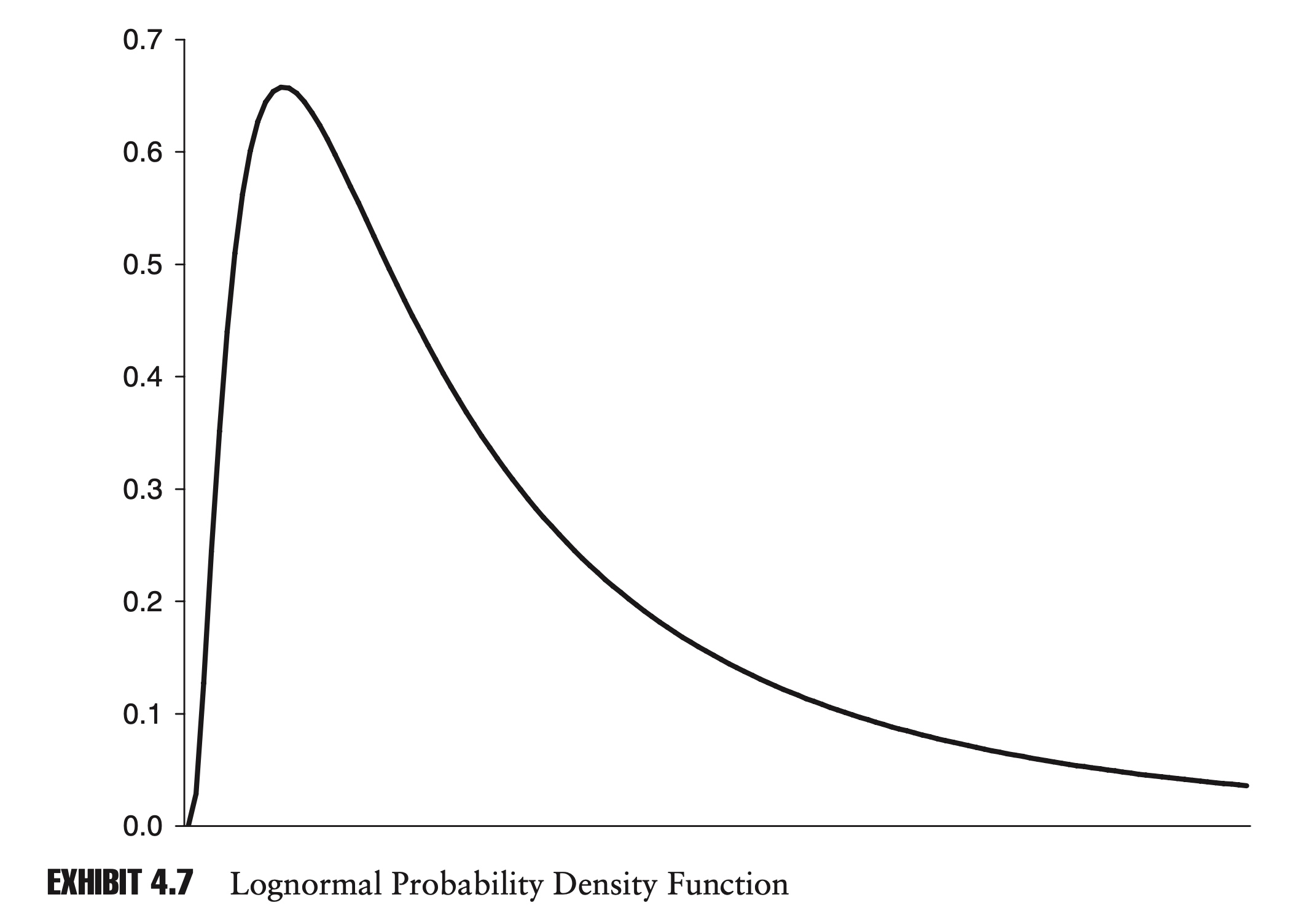
The variance of the lognormal distribution is given by:
\[E\left[(X-E[X])^{2}\right]=\left(e^{\sigma^{2}}-1\right) e^{2 \mu+\sigma^{2}}\]It is convenient to be able to describe the re- turns of a financial instrument as being lognormally distributed, rather than having to say the log returns of that instrument are normally distributed.
When it comes to modeling, though, even though they are equivalent, it is often easier to work with log returns and normal distributions than with standard returns and lognormal distributions.
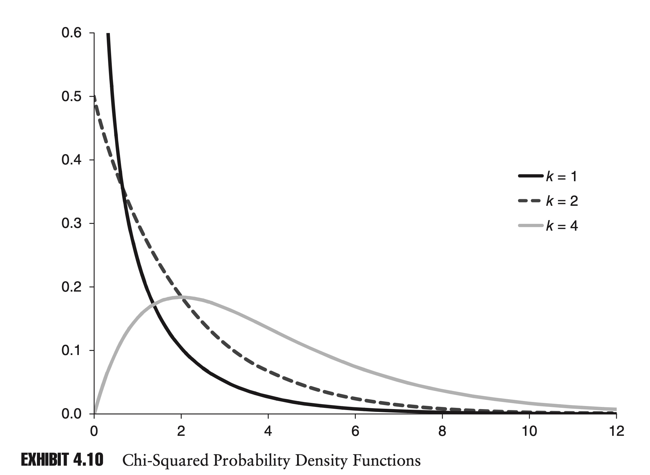
Chi-squared Distribution
If we have k independent standard normal variables, $Z_1$, $Z_2$,…, $Z_k$, then the sum of their squares, S, has a chi-squared distribution. We write:
\[\begin{array}{l} S=\sum_{i=1}^{k} Z_{i}^{2} \\ S \sim \chi_{k}^{2} \end{array}\]The variable k is commonly referred to as the degrees of freedom. It follows that the sum of two independent chi-squared variables, with k1 and k2 degrees of freedom, will follow a chi-squared distribution, with (k1 + k2) degrees of freedom.
The mean of the distribution is k, and the variance is 2k.
As k approaches infinity, the chi-squared distribution converges to the normal distribution.
For positive values of x, the probability density function for the chi-squared distribution is:
\[f(x)=\frac{1}{2^{k / 2} \Gamma(k / 2)} x^{\frac{k}{2}-1} e^{-\frac{x}{2}}\]where $\Gamma$ is the gamma function:
\[\Gamma(n)=\int_{0}^{\infty} x^{n-1} e^{-x} d x\]The chi-squared distribution is widely used in risk management, and in statistics in general, for hypothesis testing.
Student’s t Distribution
Another extremely popular distribution in statistics and in risk management is Stu- dent’s t distribution.
If Z is a standard normal variable and U is a chi-square variable with k degrees of freedom, which is independent of Z, then the random variable X,
\[X=\frac{Z}{\sqrt{U/k}}\]follows a t distribution with k degrees of freedom.
Mathematically, the distribution is quite complicated. The probability density function can be written:
\[f(x)=\frac{\Gamma\left(\frac{k+1}{2}\right)}{\sqrt{k \pi} \Gamma\left(\frac{k}{2}\right)}\left(1+\frac{x^{2}}{k}\right)^{-\frac{(k+1)}{2}}\]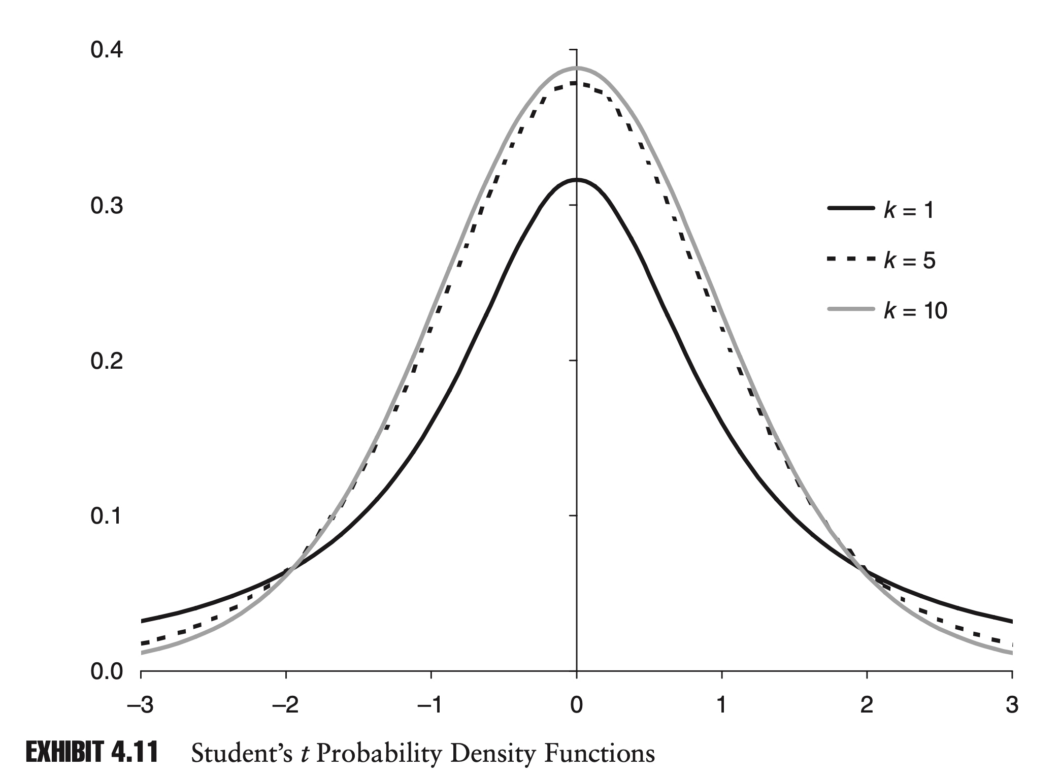
Very few risk managers will memorize this PDF equation, but it is important to understand the basic shape of the distribution and how it changes with k.
The t distribution is symmetrical around its mean, which is equal to zero. For low values of k, the t distribution looks very similar to a standard normal distribution, except that it displays excess kurtosis. As k increases, this excess kurtosis de- creases. In fact, as k approaches infinity, the t distribution converges to a standard normal distribution.
The variance of the t distribution for k > 2 is k/(k − 2). You can see that as k increases, the variance of the t distribution converges to one, the variance of the standard normal distribution.
As we will see in the following chapter, the t distribution’s popularity derives mainly from its use in hypothesis testing. The t distribution is also a popular choice for modeling the returns of financial assets, since it displays excess kurtosis.
Example:
The BLUE for population mean is the sample mean:
\[\hat{\mu}=\frac{1}{n} \sum_{i=1}^{n} r_{i}=\frac{1}{n}\left(r_{1}+r_{2}+\cdots+r_{n-1}+r_{n}\right)\]The mean and variance of this sample mean is:
\[E[\hat{\mu}]=\mu \\ V[\hat{\mu}]=\sigma^2_{\hat{\mu}} = E[(\hat{\mu}-\mu)^2]=\frac{\sigma^2}{n}\]Whereas the sample variance:
\[\begin{equation} \begin{array}{l} \hat{\sigma}^{2}=\frac{1}{n-1} \sum_{i=1}^{n}\left(x_{i}-\hat{\mu}\right) \\ E\left[\hat{\sigma}^{2}\right]=\sigma^{2} \end{array} \end{equation}\]we have
\[(n-1) \frac{\hat{\sigma}^{2}}{\sigma^{2}} \sim \chi_{n-1}^{2}\]Therefore, we can prove that \(t=\frac{\hat{\mu}-\mu}{\hat{\sigma} / \sqrt{n}}\) follow a Student’s t distribution with (n − 1) degrees of freedom.
Proof:
\[t=\frac{\frac{\hat{\mu}-\mu}{\sigma / \sqrt{n}} }{(\hat{\sigma} /\ \sigma)}\]As we know:
\[\frac{\hat{\mu}-\mu}{\sigma / \sqrt{n}} \sim N(0,1)\] \[\frac{\hat{\sigma}^{2}}{\sigma^{2}} \sim \frac{1}{n-1} \chi_{n-1}^{2}\]By definition, t follow a Student’s t distribution with (n − 1) degrees of freedom.
Common Critical Values for Student’s t Distribution:
\[\begin{array}{rrrrr} \hline & t_{10} & t_{100} & t_{1,000} & N \\ \hline 1.0 \% & -2.76 & -2.36 & -2.33 & -2.33 \\ 2.5 \% & -2.23 & -1.98 & -1.96 & -1.96 \\ 5.0 \% & -1.81 & -1.66 & -1.65 & -1.64 \\ 10.0 \% & -1.37 & -1.29 & -1.28 & -1.28 \\ 90.0 \% & 1.37 & 1.29 & 1.28 & 1.28 \\ 95.0 \% & 1.81 & 1.66 & 1.65 & 1.64 \\ 97.5 \% & 2.23 & 1.98 & 1.96 & 1.96 \\ 99.0 \% & 2.76 & 2.36 & 2.33 & 2.33 \\ \hline \end{array}\]F-distribution
If $U_1$ and $U_2$ are two independent chi-squared distributions with k1 and k2 degrees of freedom, respectively, then X
\[X=\frac{U_{1} / k_{1}}{U_{2} / k_{2}} \sim F\left(k_{1}, k_{2}\right)\]follows an F-distribution with parameters k1 and k2.
The probability density function of the F-distribution, as with the chi-squared distribution, is rather complicated:
\[f(x)=\frac{\sqrt{\frac{\left(k_{1} x\right)^{k_{1}} k_{2}^{k_{2}}}{\left(k_{1} x+k_{2}\right)^{k_{1}+k_{2}}}}}{x B\left(\frac{k_{1}}{2}, \frac{k_{2}}{2}\right)}\]where B(x, y) is the beta function:
\[B(x, y)=\int_{0}^{1} z^{x-1}(1-z)^{y-1} d z\]It is important to understand the general shape and some properties of the distribution.
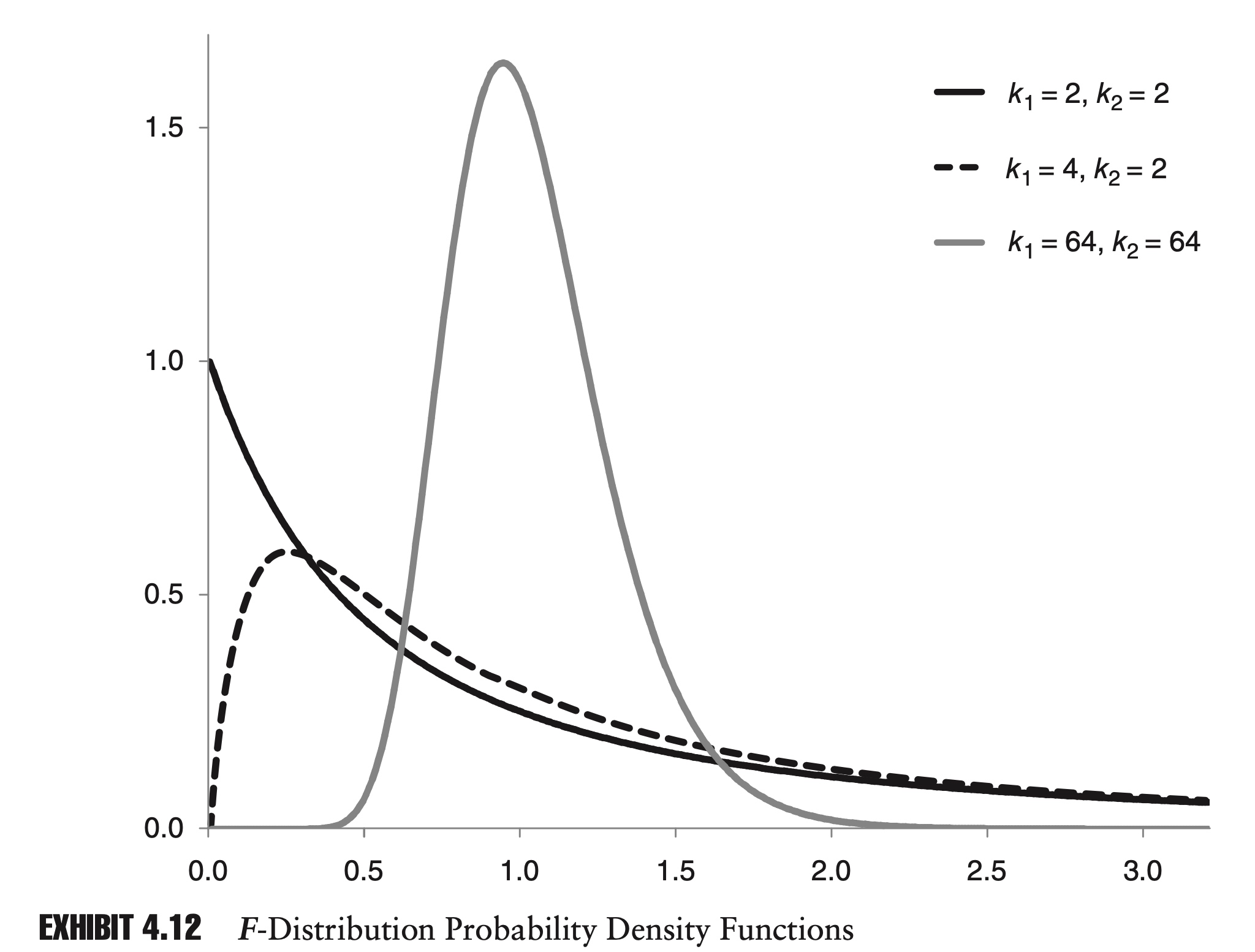
As k1 and k2 increase, the mean and mode converge to one. As k1 and k2 approach infinity, the F-distribution converges to a normal distribution.
There is also a nice relationship between Student’s t distribution and the F-distribution. From the description of the t distribution, it is easy to see that the square of a variable with a t distribution has an F-distribution.
More specifically, if X is a random variable with a t distribution with k degrees of freedom, then $X_2$ has an F-distribution with 1 and k degrees of freedom:
\[X^{2} \sim F(1, k)\]Triangular Distribution
It is often useful in risk management to have a distribution with a fixed minimum and maximum—for example, when modeling default rates and recovery rates, which by definition cannot be less than zero or greater than one.
The triangular distribution is a distribution whose PDF is a triangle. As with the uniform distribution, it has a finite range.
The PDF for a triangular distribution with a minimum of a, a maximum of b, and a mode of c is described by the following two-part function:
\[f(x)=\left\{\begin{array}{ll} \frac{2(x-a)}{(b-a)(c-a)} & a \leq x \leq c \\ \frac{2(b-x)}{(b-a)(b-c)} & c<x \leq b \end{array}\right.\]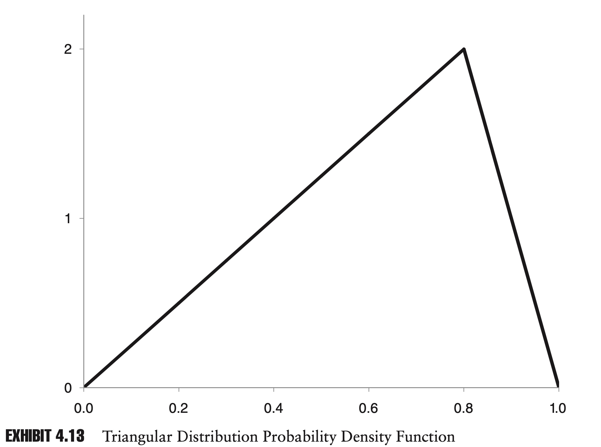
Exhibit 4.13 shows a triangular distribution where a, b, and c are 0.0, 1.0, and 0.8, respectively.
The mean, $\mu$, and variance, $\sigma^2$, of a triangular distribution are given by:
\[\begin{aligned} \mu &=\frac{a+b+c}{3} \\ \sigma^{2} &=\frac{a^{2}+b^{2}+c^{2}-a b-a c-b c}{18} \end{aligned}\]Beta Distribution
The beta distribution is another distribution with a finite range. It is more complicated than the triangular distribution mathematically, but it is also much more flexible.
The beta distribution is defined on the interval from zero to one. The PDF is defined as follows, where a and b are two positive constants:
\[f(x)=\frac{1}{B(a, b)} x^{a-1}(1-x)^{b-1} \quad 0 \leq x \leq 1\]The mean, $\mu$, and variance, $\sigma^2$, of a beta distribution are given by:
\[\begin{aligned} \mu &=\frac{a}{a+b} \\ \sigma^{2} &=\frac{a b}{(a+b)^{2}(a+b+1)} \end{aligned}\]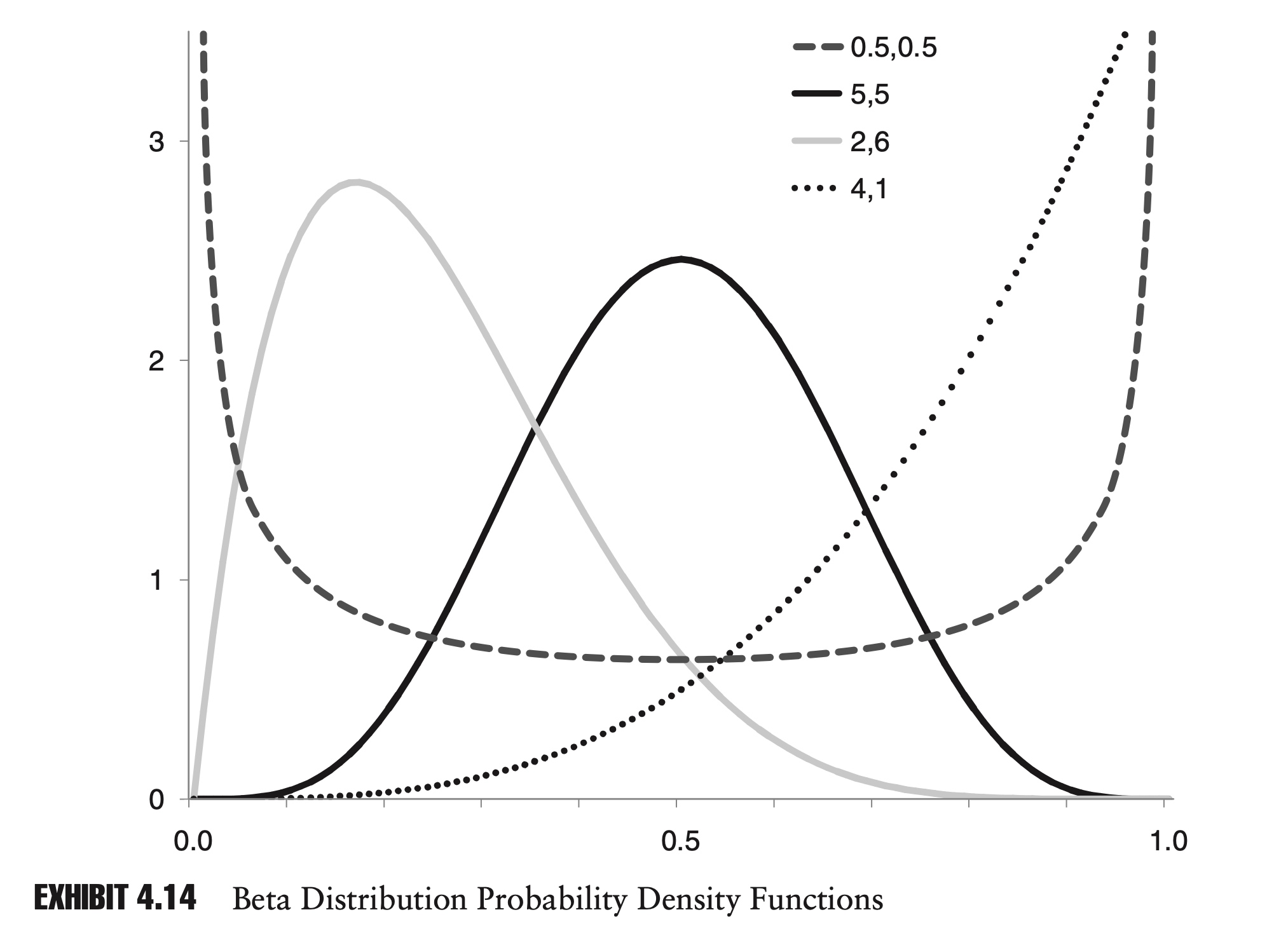
Mixture Distribution
Imagine a stock whose log returns follow a normal distribution with low volatility 90% of the time, and a normal distribution with high volatility 10% of the time.
Most of the time the world is relatively dull, and the stock just bounces along. Occasionally, though—maybe there is an earnings announcement or some other news event—the stock’s behavior is more extreme. We could write the combined density function as:
\[f(x)=w_{L} f_{L}(x)+w_{H} f_{H}(x)\]where $w_{L}$ = 0.90 is the probability of the return coming from the low-volatility distribution, $f_{L}(x)$, and $w_{H}$ = 0.10 is the probability of the return coming from the high-volatility distribution $f_{H}(x)$.
We can think of this as a two-step process.
First, we randomly choose the high or low distribution, with a 90% chance of picking the low distribution. Second, we generate a random return from the chosen normal distribution.
The final distribution, f(x), is a legitimate probability distribution in its own right, and although it is equally valid to describe a random draw directly from this distribution, it is often helpful to think in terms of this two-step process.
Note that the two-step process is not the same as the process described in a previous section for adding two random variables together. In the case we are describing now, the return appears to come from either the low-volatility distribution or the high-volatility distribution.
The distribution that results from a weighted average distribution of density functions is known as a mixture distribution. More generally, we can create a distribution:
\[f(x)=\sum_{i=1}^{n} w_{i} f_{i}(x) \text { s.t. } \sum_{i=1}^{n} w_{i}=1\]Mixture distributions are extremely flexible. In a sense they occupy a realm between parametric distributions and nonparametric distributions.
In a typical mixture distribution, the component distributions are parametric, but the weights are based on empirical data, which is nonparametric.
Just as there is a trade-off between parametric distributions and nonparametric distributions, there is a trade- off between using a low number and a high number of component distributions.
By adding more and more component distributions, we can approximate any data set with increasing precision. At the same time, as we add more and more component distributions, the conclusions that we can draw tend to become less general in nature.—- Variance VS Underfitting problem
Just by adding two normal distributions together, we can develop a large number of interesting distributions.
- Similar to the previous example, if we combine two normal distributions with the same mean but different variances, we can get a symmetrical mixture distribution that displays excess kurtosis.
- By shifting the mean of one distribution, we can also create a distribution with positive or negative skew.
- Finally, if we move the means far enough apart, the resulting mixture distribution will be bimodal; that is, the PDF will have two distinct maxima,
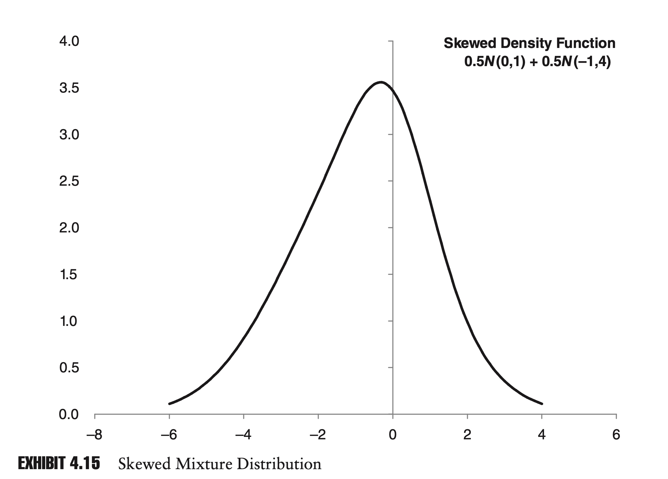
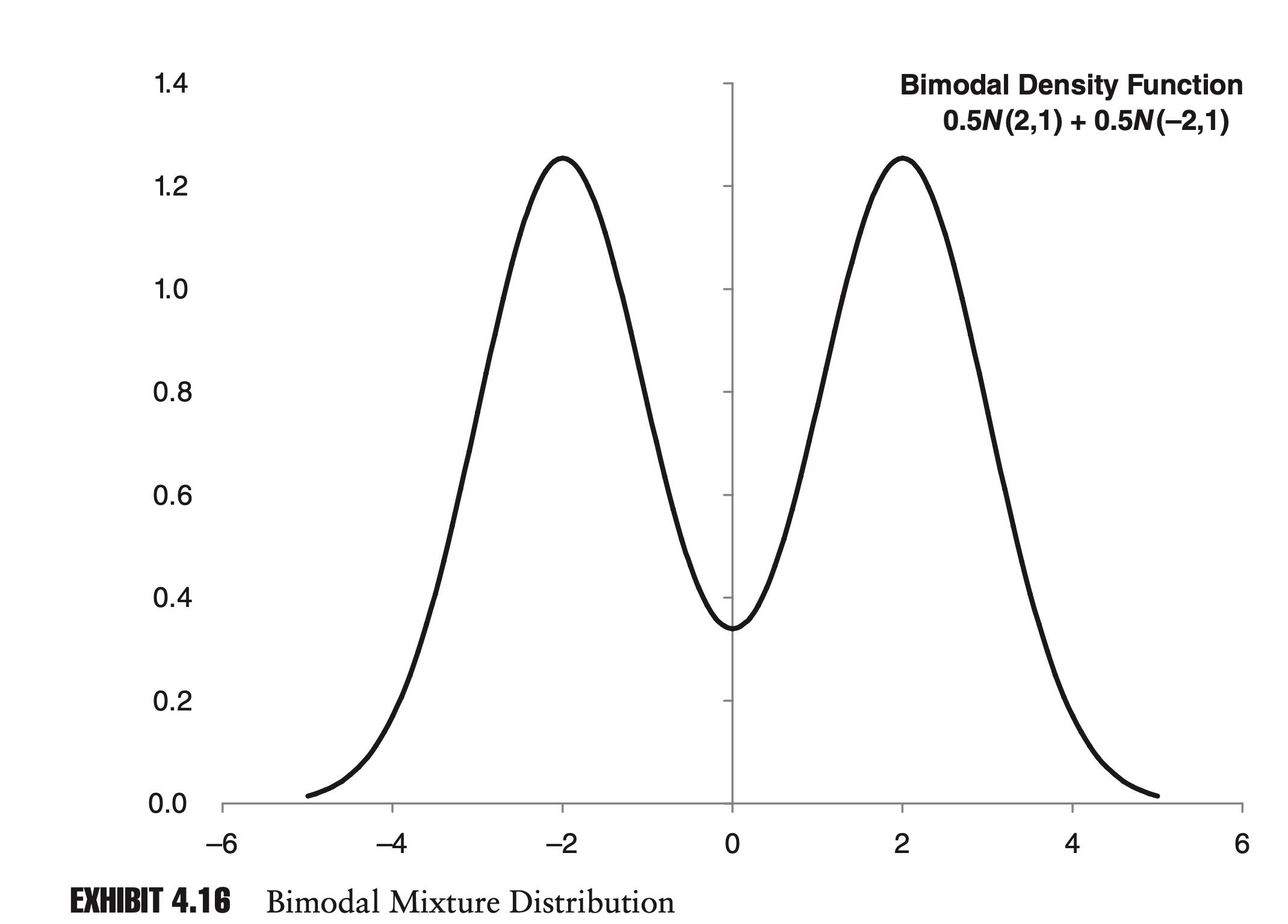
Mixture distributions can be extremely useful in risk management. Securities whose return distributions are skewed or have excess kurtosis are often considered riskier than those with normal distributions, since extreme events can occur more frequently. Mixture distributions provide a ready method for modeling these attributes.
Chapter 3: Copulas
In this chapter we explore distributions involving more than one variable, and pro- vide a brief overview of copulas. Multivariate distributions are an important tool for modeling portfolios.
In everyday parlance, a copula is simply something that joins or couples. In statistics, a copula is a function used to combine two or more cumulative distribution functions in order to produce one joint cumulative distribution function.
A copula only defines a relationship between univariate distributions. The underlying distributions themselves can be any shape or size.
Mechanically, copulas take as their inputs two or more cumulative distributions and output a joint cumulative distribution. The advantage of working with cumulative distributions is that the range is always the same. No matter what the distribution is, the output of a cumulative distribution always ranges from 0% to 100%.
Say we have two random variable X and Y, with the cumulative distribution function as $u=F_X(x)$ and $v=F_Y(y)$.
A copula gives a joint cumulative distribution function as $C(u,v)$ s.t.:
\[\begin{aligned} C(1,1) &=1 \\ C(0,0) &=0\\ \frac{\partial C }{\partial u} &\geq 0\\ \frac{\partial C }{\partial v} &\geq 0 \end{aligned}\]For example, given two cumulative distributions, u and v, and a constant, $\alpha$, we can write Frank’s copula as:
\[C(u, v)=\frac{1}{\alpha} \ln \left[1+\frac{\left(e^{\alpha u}-1\right)\left(e^{\alpha v}-1\right)}{e^{\alpha}-1}\right]\]To calculate the joint PDF (probability density function) of a copula, we can use the chain rule:
\[f(x, y)=\frac{\partial^{2} C(u, v)}{\partial x \partial y}=\frac{\partial^{2} C(u, v)}{\partial u \partial v} \frac{\partial u}{d x} \frac{\partial v}{d y}=c(u, v) f(x) f(y)\]Here we have denoted the second cross partial derivative of $C(u,v)$ by $c(u,v)$. $c(u,v)$ is often referred to as the density function of the copula. Because $c(u,v)$ depends on only the copula and not the marginal distributions, we can calculate $c(u,v)$ once and then apply it to many different problems.
If we work on the x-y space, we should have
\[\begin{aligned} \int_x \int_y f(x,y)dxdy=1 \end{aligned}\]since
\[\begin{aligned} du&=f_X(x)dx\\ dv&=f_Y(y)dy \end{aligned}\]we have:
\[\begin{aligned} \int_0^1 \int_0^1 c(u,v)dudv=1 \end{aligned}\]Moreover, since that u and v are both uniformly distributed in [0,1], we know that the marginal PDF is always $I_{[0,1]}$.
In other words, for \(\forall u^*,v^*\), we must have
\[\begin{aligned} \int_0^1 c(u^*,v)dv&=1\\ \int_0^1 c(u,v^*)du&=1 \end{aligned}\]In summary, a copulas $C(u,v)$ is defined by
\[C(u^*,v^*)=\int_0^{u^*} \int_0^{v^*} c(u,v)dvdu\]where $c(u,v): [0,1]\times[0,1] \to [0,+\infty) $ satisfies
\[\begin{aligned} \int_0^1 c(u^*,v)dv&=1\\ \int_0^1 c(u,v^*)du&=1 \end{aligned}\]Steps to calculate the PDF of a copula
Step 1:
For any point on the graph, (x,y), we first calculate values for both the PDF and the CDF of X and Y.
Step 2:
Use the CDF (u,v) of X and Y at (x,y), we can calculate the $c(u,v)$.
Step 3:
\[\begin{aligned} f(x, y)&=c(u, v)f(x) f(y) \\ c(u, v)&=\frac{\partial^{2} C(u, v)}{\partial u \partial v} \end{aligned}\]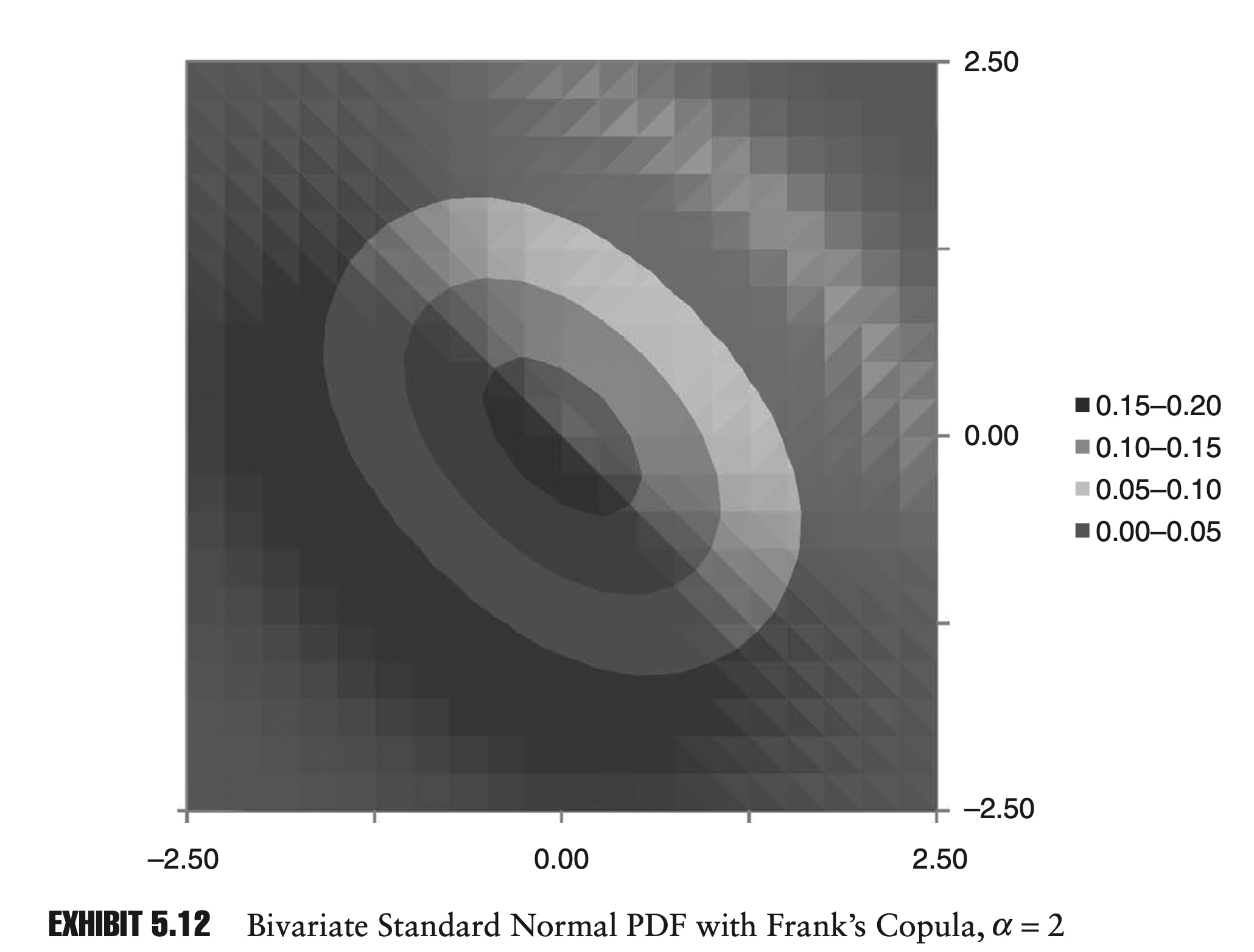
Using Copulas in simulations
In this section, we demonstrate how copulas can be used in Monte Carlo simulations.
In order to use copulas in a Monte Carlo simulation, we need to calculate the inverse marginal CDFs for the copula.
To determine the marginal CDFs of a copula, we take the first derivative of the copula function with respect to one of the under- lying distributions. For two cumulative distributions u and v, the marginal CDFs would be:
\[C(u^*,v^*)=\int_0^{u^*} \int_0^{v^*} c(u,v)dv du\] \[\begin{array}{l} C_{1}(u^*,v^*)=\frac{\partial C}{\partial u}(u^*,v^*)=\int_0^{v^*} c(u^*, v) d v \\ C_{2}(u^*,v^*)=\frac{\partial C}{\partial v}(u^*,v^*)=\int_0^{u^*} c(u, v^*) d u \end{array}\]Note that \(c(u^*, v)\) is the conditional PDF for \(v^* \in [0,1]\):
\[\int_0^{1} c(u^*, v) d v=1\]As a result, $C_1$ is a conditional CDF for \(v^*\). Therefore, under the condition that \(u=u^*\), \(C_1(u^*, v^*)\) is uniformly distributed on $[0,1]$.
For example, for Frank’s copula the marginal CDF for u would be:
\[C_{1}=\frac{\partial C}{\partial u}=\frac{\left(e^{-\alpha u}-1\right)\left(e^{-\alpha v}-1\right)+\left(e^{-\alpha v}-1\right)}{\left(e^{-\alpha u}-1\right)\left(e^{-\alpha v}-1\right)+\left(e^{-\alpha}-1\right)}\]$C_1$ is a proper CDF, and varies between 0% and 100%. To determine the inverse of $C_1$, we solve for $v$:
\[v=-\frac{1}{\alpha} \ln \left[1+\frac{C_{1}\left(e^{-\alpha}-1\right)}{1+\left(e^{-\alpha u}-1\right)\left(1-C_{1}\right)}\right]\]Each iteration in the Monte Carlo simulation then involves three steps:
- Generate two independent random draws from a standard uniform distribution. These are the values for $u$ and $C_1$.
- Use the inverse CDF of the copula to determine v. This is the essential step. Depending on the copula, different values of v will be more or less likely, given u.
- Calculate values for x and y, using inverse cumulative distribution functions for the underlying distributions. For example, if the underlying distributions are normal, use the inverse normal CDF to calculate x and y based on u and v.
Parameterization of Copulas
Given a copula, we know how to calculate values for that copula, but how do we know which copula to use in the first place? The answer is a mixture of art and science.
If the data seem to exhibit increased correlation in crashes, then you should choose a copula that displays a higher probability in the negative-negative region such as the Clayton copula.
Once we know which type of copula we are going to use, we need to determine the parameters of the copula. Take for example the Farlie-Gumbel-Morgenstern (FGM) copula, given by:
\[C=uv[1+\alpha (1-u)(1-v)]\]We can prove that
\[c(u,v)=1+\alpha-2\alpha u -2\alpha v +4 \alpha uv\]As with most copulas, there is a single parameter, α, which needs to be determined, and this parameter is related to how closely the two underlying random variables are related to each other.
In statistics, the popular methods for measuring how closely two variables are related to each other include:
1) Pearson’s correlation or linear correlation
\[\text { Correlation }=\frac{E[(X-E[X])(Y-E[Y])]}{\sigma_{X} \sigma_{Y}}\]2) Kendall’s tau
If we have $(X_i-X_j)(Y_i - Y_j)>0 $, we say that the two points are concordant.
Kendall’s tau is defined as the probability of concordance minus the probability of discordance.
\[\tau = P[\text{concordance}] – P[\text{discordance}]\]If P[concordance] is 100%, then P[discordance] must be 0%. Similarly, if P[discordance] is 100%, P[concordance] must be 0%. Because of this, like our standard correlation measure, Kendall’s tau must vary between −100% and +100%.
\[\tau=\frac{\text{# of concordant pairs − # of discordant pairs}}{C_n^2}\]Characteristics of Kendall’s tau:
- It is less sensitive to outliers than Pearson’s correlation.
- Measures of dependence based on rank are in- variant under strictly increasing transformations
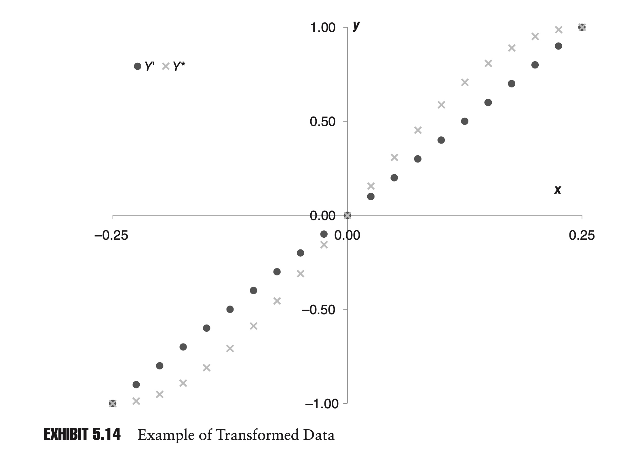
As long as the transformation does not change the relative order of the points, Kendall’s tau won’t change, while the Linear Correlation changes.
This propostion suggests that, at least for Kendall’s tau, the “correlation” X and Y is equal to the “correlation” between U(X) and V(Y). In otherwords, the Kendall’s tau will only be determined by the U and V, and the marginal distribution does not matter any more.
As it turns out, for many copulas, changing the value of the shape parameter, α, will transform the data in a way that is similar to the way the data was transformed in Exhibit 5.14.
Changing α will change the shape of the data, but it will not change the order. For a given type of copula, then, Kendall’s tau is often a function of the copula’s parameter, α, and does not depend on what type of marginal distributions are being used.
This leads to a simple method for setting the parameter of the copula. First, calculate Kendall’s tau, and then set the shape parameter based on the appropriate formula for that copula relating Kendall’s tau and the shape parameter.
Given an equation for a copula, C(u,v) and its density function c(u,v), Kendall’s tau can be determined as follows:
\[\tau=4 E[C(u, v)]-1=4 \int_{0}^{1} \int_{0}^{1} C(u, v) c(u, v) d u d v-1\]3) Spearman’s rho
To calculate Spear- man’s rho from sample data, we simply calculate our standard correlation measure using the ranks of the data.
We can also calculate Spearman’s rho from a copula function:
\[\rho_{s}=12 \int_{0}^{1} \int_{0}^{1} C(u, v) d u d v-3\]Rather than being based directly on the values of the variables, both Kendall’s tau and Spearman’s rho are based on the order or rank of the variables.
Comments