t location-scale model
For many financial data, it turns out the historical logreturns often can not be approximated well by a normal distribution. In fact, the heavy-tails effect and the higher density near the mean can not be caputred by $N(\mu,\sigma)$.
Luckily, we can use t location-scale model to capture all these missing characteristics. Before we jump into the defintion and application of this model, we have to revisit the student-t distribution.
student’s t-distribution
We can define student-t distribution through two approach.
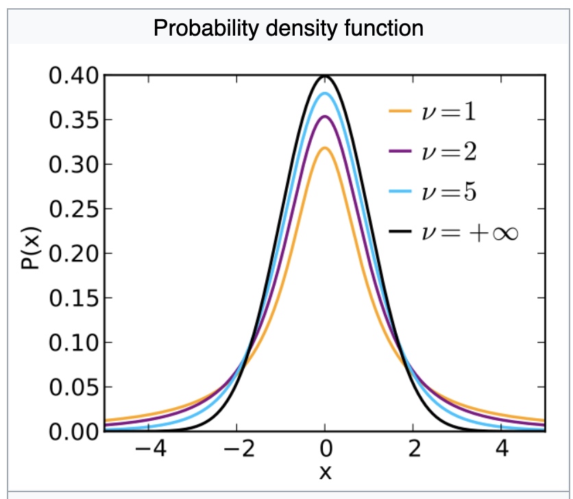
Student’s t-distribution has the probability density function given by:
\[f(t)=\frac{\Gamma\left(\frac{\nu+1}{2}\right)}{\sqrt{\nu \pi} \Gamma\left(\frac{\nu}{2}\right)}\left(1+\frac{t^{2}}{\nu}\right)^{-\frac{\nu+1}{2}}\]where $\nu $ is the number of degrees of freedom and $\Gamma$ is the gamma function.
Statistics
When $0<dof<=1$, all moments are undefined.
The theoretical statistics (i.e., in the absence of sampling error) when $dof>1$ are as follows.
- Mean=Mode=Median=0
- \[Variance = \begin{cases} \infty, & \text{if $v\leq$ 2} \\ \frac{v}{v-2}, & \text{if $v>$ 2} \end{cases}\]
- Skewness=0 if v>3
- \[Kurtosiso = \begin{cases} \infty, & \text{if $2<v\leq4$ } \\ 3+\frac{6}{v-4}, & \text{if $v>4$} \end{cases}\]
t Location-Scale Distribution
The t location-scale distribution is useful for modeling data distributions with heavier tails (more prone to outliers) than the normal distribution. It approaches the normal distribution as ν approaches infinity, and smaller values of ν yield heavier tails.
A t Location-Scale Distributed random variable has 3 parameters $(\mu,\sigma,\nu)$, and can be defined as:
\[r=\mu + \sigma* T(\nu)\]If we set
\[\sigma =\sqrt{\frac{v-2}{v}}\]r will have a variance of 1, and now it is called as a rescaled t-distribution
Here is how the rescaled t-distribution changes as the degree of freedom increases.
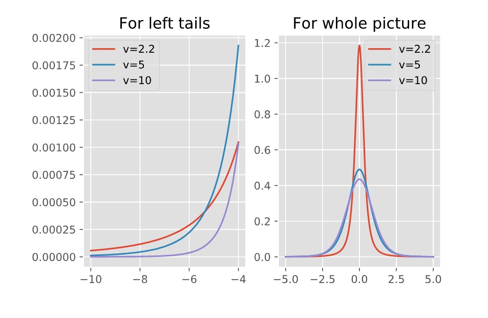
As we can see, when $nu$ is smaller:
- near the mean: the probability density function will be higher than “normal”
- the left and right tails: the PDF will also be higher than “normal”, which means fat tails
Codes in Python
histogram visualization
Draw the histogram and the PDF for fitted t location-scale and normal distribution.
1
2
3
4
5
6
7
8
9
10
11
12
13
14
15
16
17
18
19
20
21
22
23
24
25
26
27
28
29
30
31
32
33
34
35
36
37
38
39
40
41
42
43
44
45
46
47
48
49
50
51
52
53
54
55
def myhist(df_input, bins=30):
    import matplotlib.pyplot as plt
    import matplotlib.style as style
    import scipy.stats as stats
    import numpy as np

    df_input = np.array(df_input)
    if df_input.ndim > 1:
        if df_input.shape[0] > 1:
            df_input = df_input[:, 0]
        else:
            df_input = df_input[0, :]

    style.use("ggplot")
    plt.rcParams["figure.figsize"] = (6, 4)
    plt.figure(dpi=100)
    heightofbins, aa, bb = plt.hist(df_input, bins)
    mu = df_input.mean()
    std = df_input.std()
    lowb = df_input.min()
    upb = df_input.max()

    # can use stats.norm.fit to get the std, mu
    # nloc,nscale=stats.norm.fit(df_input)

    # fit the data with a t location-scale model with MLE
    ## r=loc + scale * T(dof)

    tdof, tloc, tscale = stats.t.fit(df_input)

    # Change the shape of PDF to match the hist
    ## both norm and t distribution pdf are multiplied by a same number

    ### norm distribution
    xx = stats.norm.pdf(np.linspace(lowb - std, upb + std, 1000), loc=mu, scale=std)
    xx = xx * np.max(heightofbins) / stats.t.pdf(mu, df=tdof, loc=tloc, scale=tscale)
    plt.plot(np.linspace(lowb - std, upb + std, 1000), xx)

    ### rescaled t distribution
    y = stats.t.pdf(
        np.linspace(lowb - std, upb + std, 1000), df=tdof, loc=tloc, scale=tscale
    )
    y = y * np.max(heightofbins) / stats.t.pdf(mu, df=tdof, loc=tloc, scale=tscale)
    plt.plot(np.linspace(lowb - std, upb + std, 1000), y)

    plt.legend(["Normal PDF", "Rescaled t Distribution", "Sample Distribution"])

    ### plot the sample kurtosis and skewness
    kur = stats.kurtosis(df_input)
    skew = stats.skew(df_input)
    x = mu + std
    y = 0.5 * np.max(heightofbins)
    plt.text(x, y, "Skewness:{:.2f},Kurtosis:{:.2f}".format(skew, kur))
    plt.show()
Value at risk
The following function can calculate the Var_001, Var_005 for given data. It has 3 different methods to derive the vars:
- norm
- t
- historical
1
2
3
4
5
6
7
8
9
10
11
12
13
14
15
16
17
18
19
20
21
22
23
24
25
26
27
28
29
30
31
32
33
34
35
36
37
38
39
40
41
42
43
44
45
46
47
48
49
50
51
52
53
54
55
56
57
58
59
60
61
62
63
64
65
66
67
68
69
70
71
72
73
74
75
76
77
78
79
80
81
82
83
84
85
86
87
88
89


def myvar(df_input, alphas=[0.01, 0.05], method="all", tell=True):
    if method not in ["all", "norm", "t", "historical"]:
        print("Fail: wrong method! Please use one of the following method:")
        for i in ["all", "norm", "t", "historical"]:
            print(i)
        return "Error"
    import matplotlib.pyplot as plt
    import matplotlib.style as style
    import scipy.stats as stats
    import numpy as np

    alphas = np.array(alphas)

    try:
        palphas = [item * 100 for item in alphas]
    except:
        palphas = 100 * alphas

    df_input = np.array(df_input)
    if df_input.ndim > 1:
        if df_input.shape[0] > 1:
            df_input = df_input[:, 0]
        else:
            df_input = df_input[0, :]

    # parametric method with norm distribution
    # Analytic Approach
    if method == "norm" or method == "all":
        nloc, nscale = stats.norm.fit(df_input)
        vars = stats.norm.ppf(alphas, loc=nloc, scale=nscale)
        if tell == True or method == "all":
            print("Use Norm-Distribution model:")
            try:
                for var, alpha in zip(vars, alphas):
                    print("Var {}: \t{} ".format(alpha, var))
            except:
                for var, alpha in zip([vars], [alphas]):
                    print("Var {}: \t{} ".format(alpha, var))

        if method != "all":
            return vars

    # parametric method with t location-scale distribution
    # fit the data with a t location-scale model with MLE
    ## r=loc + scale * T(dof)

    if method == "t" or method == "all":
        tdof, tloc, tscale = stats.t.fit(df_input)
        vars = stats.t.ppf(alphas, df=tdof, loc=tloc, scale=tscale)
        if tell == True or method == "all":
            print("Use t location-scale model:")
            try:
                for var, alpha in zip(vars, alphas):
                    print("Var {}: \t{} ".format(alpha, var))
            except:
                for var, alpha in zip([vars], [alphas]):
                    print("Var {}: \t{} ".format(alpha, var))

        if method != "all":
            return vars

    # historical method
    if method == "historical" or method == "all":
        vars = np.percentile(df_input, palphas)
        if tell == True or method == "all":
            print("Use Historical Approach:")
            try:
                for var, alpha in zip(vars, alphas):
                    print("Var {}: \t{} ".format(alpha, var))
            except:
                for var, alpha in zip([vars], [alphas]):
                    print("Var {}: \t{} ".format(alpha, var))

        if method != "all":
            return vars


if __name__ == "__main__":

    print("This is my Var module")
    import scipy.stats as stats
    df = stats.t.rvs(df=5, scale=2, size=10000, loc=0)
    myvar(df,alphas=[0.01,0.05,0.1])
    xx = stats.t.ppf(df=5, scale=2, loc=0, q=[0.01, 0.05, 0.1])
    print("Real Vars:")
    print(xx)
Espected Shortfall
1
2
3
4
5
6
7
8
9
10
11
12
13
14
15
16
17
18
19
20
21
22
23
24
25
26
27
28
29
30
31
32
33
34
35
36
37
38
39
40
41
42
43
44
45
46
47
48
49
50
51
52
53
54
55
56
57
58
59
60
61
62
63
64
65
66
67
68
69
70
71
72
73
74
75
76
77
78
79
80
81
82
83
84
85
86
87
88
89
90
91
92
93
94
95
96
97
98
99
def myes(df_input, alphas=[0.01, 0.05], num_of_simus=1000000, method="all", tell=True):
    if method not in ["all", "norm", "t", "historical"]:
        print("Fail: wrong method! Please use one of the following method:")
        for i in ["all", "norm", "t", "historical"]:
            print(i)
        return "Error"

    import matplotlib.pyplot as plt
    import matplotlib.style as style
    import scipy.stats as stats
    import numpy as np

    alphas = np.array(alphas)

    try:
        palphas = [item * 100 for item in alphas]
    except:
        palphas = 100 * alphas

    df_input = np.array(df_input)
    if df_input.ndim > 1:
        if df_input.shape[0] > 1:
            df_input = df_input[:, 0]
        else:
            df_input = df_input[0, :]

    # parametric method with norm distribution
    if method == "norm" or method == "all":
        nloc, nscale = stats.norm.fit(df_input)
        vars = stats.norm.ppf(alphas, loc=nloc, scale=nscale)
        nrvs = stats.norm.rvs(loc=nloc, scale=nscale, size=num_of_simus)
        try:
            ess = [nrvs[nrvs < var].mean() for var in vars]
        except:
            ess = nrvs[nrvs < vars].mean()
        if tell == True or method == "all":
            print("Use Analytical Norm-Distribution model:")
            try:
                for es, alpha in zip(ess, alphas):
                    print("ES {}: \t{} ".format(alpha, es))
            except:
                for es, alpha in zip([ess], [alphas]):
                    print("ES {}: \t{} ".format(alpha, es))
        if method != "all":
            return ess

    # parametric method with t location-scale distribution
    # fit the data with a t location-scale model with MLE
    ## r=loc + scale * T(dof)

    if method == "t" or method == "all":
        tdof, tloc, tscale = stats.t.fit(df_input)
        vars = stats.t.ppf(alphas, df=tdof, loc=tloc, scale=tscale)
        trvs = stats.t.rvs(df=tdof, scale=tscale, size=num_of_simus, loc=tloc)
        try:
            ess = [nrvs[nrvs < var].mean() for var in vars]
        except:
            ess = nrvs[nrvs < vars].mean()

        if tell == True or method == "all":
            print("Use Analytical t location-scale model:")
            try:
                for es, alpha in zip(ess, alphas):
                    print("ES {}: \t{} ".format(alpha, es))
            except:
                for es, alpha in zip([ess], [alphas]):
                    print("ES {}: \t{} ".format(alpha, es))
        if method != "all":
            return ess

    # historical method
    if method == "historical" or method == "all":
        vars = np.percentile(df_input, palphas)
        try:
            ess = [nrvs[nrvs < var].mean() for var in vars]
        except:
            ess = nrvs[nrvs < vars].mean()
        if tell == True or method == "all":
            print("Use Historical Approach:")
            try:
                for es, alpha in zip(ess, alphas):
                    print("ES {}: \t{} ".format(alpha, es))
            except:
                for es, alpha in zip([ess], [alphas]):
                    print("ES {}: \t{} ".format(alpha, es))
        if method != "all":
            return ess


if __name__ == "__main__":

    print("This is my Expected Shortfall module")
    import scipy.stats as stats

    # for calculating ES, we only have 1% or 5% useful data, therefore we want to increase the number of simulations
    df = stats.t.rvs(df=5, scale=2, size=10000, loc=0)

    myes(df, num_of_simus=10000000, alphas=[0.01, 0.05, 0.1])
Application
1
2
3
4
5
6
7
8
9
10
11
12
13
14
15
16
17
18
19
20
21
22
23
24
25
26
27
28
29
30
31
32

if __name__ == "__main__":

    print("This is my first module")

    from WindPy import w
    import scipy.stats as stats

    w.start()  # 默认命令超时时间为120秒,如需设置超时时间可以加入waitTime参数,例如waitTime=60,即设置命令超时时间为60秒

    print("WindPy是否已经登录成功:{}".format(w.isconnected()))  # 判断WindPy是否已经登录成功

    eroc, df = w.wsd("USDCNY.EX", "close", "2010-01-01",
                     "2020-12-28", usedf=True)
    myhist(df.diff().dropna(), bins=100)
    myvar(df.diff().dropna(), method="t", tell=True)
    import pandas as pd

    df.index = pd.to_datetime(df.index)
    for i in range(2015, 2021):
        print("For year {}:".format(i))
        [var1, var2] = myvar(
            -df[df.index.year == i].diff().dropna(), method="t", tell=False
        )
        print("Var_001={:.5f}, Var_005={:.5f}".format(var1, var2))
        parameters = stats.t.fit(-df[df.index.year == i].diff().dropna())
        print("DF={}\t Loc={}\t Scale={}".format(*parameters))
        print("The stats are:")
        statistics = stats.t.stats(*parameters, moments="mvsk")
        print("Mean={}\t Variance={}\t Skew={}\t Kurtosis={}".format(*statistics))
        print("-------------------------------------------")
Comments