Risk factors
Risk management systems are based on models that describe potential changes in the factors affecting portfolio value.
In other words, RM models function as:
\[\begin{aligned} \text{Risk fators} \to \text{Prices of Instruments} \to \text{P&L of Portfolios} \end{aligned}\]By generating future scenarios for each risk factor, we can infer changes in portfolio value and reprice the portfolio accordingly for different “states of the world.”
Method 1 is similar to Bayesian Analysis in the sense that, we assume a distribution function for the risk factor before we incorporating the past information. Therefore, the past information is only used to calibrate the parameters of the distribution function.
Method 2, however, totally relies on the past information, and bears no prior belief.
Predict risk factors: with Models based on Distributional Assumptions
Classic methodology presented in RiskMetrics Classic
In the classic methodology presented in RiskMetrics Classic, a distribution function is assumed for the log-return of the risk factors. This prior distribution is indeed called conditionally normal distribution. Here is the definition:
Moreover, the classic model updates the return volatility estimates based on the arrival of new information, where the importance of old observations diminishes exponentially with time.
The model for the distribution of future returns is based on the notion that log-returns, when standardized by an appropriate measure of volatility, are independent across time and normally distributed.
How to get calibrate the conditionally normal distribution
With this so-called “conditionally normal distribution” in our mind, we still need to estimate the volatility and correlation of the risk factors before we can apply this model.
Luckily, information about volatility and correlation are all included in the covariance matrix! It means we just need to estimate the covariance matrix $\sum $ for the risk factors.
For single risk factor model
Let us start by defining the logarithmic return of a risk factor as
\[r_{t, T}=\log \left(\frac{P_{T}}{P_{t}}\right)=p_{T}-p_{t}\]where $r_{t, T}$ denotes the logarithmic return from time t to time T. $P_T$ is the level/price of the risk factor, $p_t=log(P_T )$ is the log-price.
Given a volatility estimate $\sigma$, the process generating the returns follows a geometric random walk:
\[\frac{dP_t}{P_t}=\mu dt + \sigma dW_t\]By Ito’s formula, this means that the return from time t to time T can be written as:
\[r_{t, T}=\left(\mu-\frac{1}{2} \sigma^{2}\right)(T-t)+\sigma \varepsilon \sqrt{T-t} \tag{1}\label{1}\]where $\varepsilon \sim N (0, 1)$.
There are two parameters that need to be estimated in \eqref{1}: the drift $\mu$ and the volatility $\sigma$.
In other words, when we are dealing with short horizons, using a zero expected return assumption is as good as any mean estimate one could provide, except that we do not have to worry about producing a number for $\mu$. Hence, from this point forward, we will make the explicit assumption that the expected return is zero, or equivalently that $\mu=\frac{1}{2}\sigma^2$ .
We can incorporate the zero mean assumption in \eqref{1} and express the return as
\[r_{t, T}=\sigma \varepsilon \sqrt{T-t} \tag{2}\label{2}\]The next question is how to estimate the volatility $\sigma$.
We use an exponentially weighted moving average (EWMA) of squared returns as an estimate of the volatility. If we have a history of m + 1 one-day returns from time t − m to time t , we can write the one-day volatility estimate at time t as
\[\sigma=\frac{1-\lambda}{1-\lambda^{m+1}} \sum_{i=0}^{m} \lambda^{i} r_{t-i}^{2}=R^{\top} R\]where $0<λ≤1$ is the decay factor,$r_t$ denotes the return from day t to day t+1, and
\[R=\sqrt{\frac{1-\lambda}{1-\lambda^{m+1}}}\left(\begin{array}{c} r_{t} \\ \sqrt{\lambda} r_{t-1} \\ \vdots \\ \sqrt{\lambda^{m}} r_{t-m} \end{array}\right)\]How to estimate the decay factor
By using the idea that the magnitude of future returns corresponds to the level of volatility, one approach to select an appropriate decay factor is to compare the volatility obtained with a certain λ to the magnitude of future returns.
According to RiskMetrics Classic, we formalize this idea and obtain an optimal decay factor by minimizing the mean squared differences between the variance estimate and the actual squared return on each day. Using this method, it is showed that each time series (corresponding to different countries and asset classes), has a different optimal decay factor ranging from 0.9 to 1.
In addition, is is found that the optimal λ to estimate longer-term volatility is usually larger than the optimal λ used to forecast one-day volatility.
The conclusion of the discussion in RiskMetrics Classic is that on average λ = 0.94 produces a very good forecast of one-day volatility, and λ = 0.97 results in good estimates for one-month volatility.
It is worth mentioning that, the information captured with decay factor $\lambda $ and number of observation $m$ is:
\[1-\lambda ^m\]If we take m to the limit, we can prove that
\[\sigma^2_t=\lambda \sigma^2_{t-1}+(1-\lambda)r_t^2\]Conditional normal distribution may produce heavy-tails
The assumption behind this model is that one-day returns conditioned on the current level of volatility are independent across time and normally distributed. It is important to note that this assumption does not preclude a heavy-tailed unconditional distribution of returns.
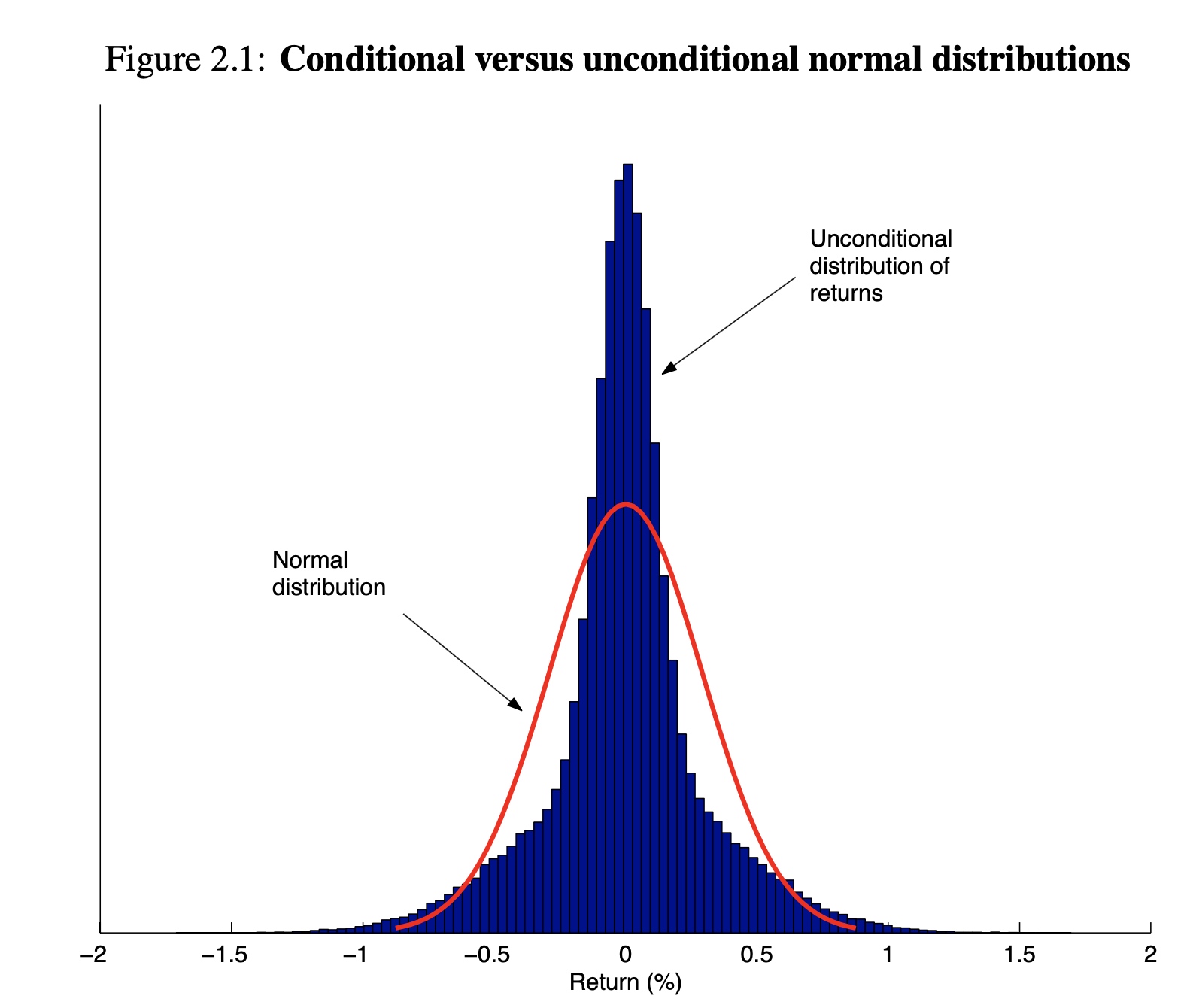
Figure 2.1 compares the unconditional distribution of returns described above to a normal distribution with the same unconditional volatility. One can see that the unconditional distribution of returns has much heavier tails than those of a normal distribution.
For multiple risk factor model
Suppose that we have n risk factors. Then, the process generating the returns for each risk factor can be written as
\[\frac{d P_{t}^{(i)}}{P_{t}^{(i)}}=\mu_{i} d t+\sigma_{i} d W_{t}^{(i)}, \quad i=1, \ldots, n \tag{3}\label{3}\]where $Var(dW^{(i)})=dt, Cov(dW^{(i)},dW^{(j)})=\rho_{i,j}d_t$.
From \eqref{3} it follows that the return on each asset from time t to time t + T can be written as
\[r_{t, T}^{(i)}=\left(\mu_{i}-\frac{1}{2} \sigma_{i}^{2}\right)(T-t)+\sigma_{i} \varepsilon_{i} \sqrt{T-t}\]where $\varepsilon_i \sim N (0, 1)$ and $Cov[\varepsilon_i,\varepsilon_j]=\rho_{i,j}$.
If we incorporate the zero mean assumption we get that
\[r_{t, T}^{(i)}=\sigma_{i} \varepsilon_{i} \sqrt{T-t}\]Then with EWMA model for estimation of covariances, the covariance between returns on asset i and asset j can be written as:
\[{\sum}_{i,j}=\sigma_i \sigma_j \rho_{i,j}=\frac{1-\lambda}{1-\lambda^{m+1}} \sum_{k=0}^{m} \lambda^{k} r_{t-k}^{(i)}r_{t-k}^{(j)}\]We can also write the covariance matrix as
\[\sum=R^T R\]where R is an m × n matrix of weighted returns:
\[R=\sqrt{\frac{1-\lambda}{1-\lambda^{m+1}}}\left(\begin{array}{cccc} r_{t}^{(1)} & r_{t}^{(2)} & \cdots & r_{t}^{(n)} \\ \sqrt{\lambda} r_{t-1}^{(1)} & \cdots & \cdots & \sqrt{\lambda} r_{t-1}^{(n)} \\ \vdots & \vdots & \vdots & \vdots \\ \vdots & \vdots & \vdots & \vdots \\ \sqrt{\lambda^{m}} r_{t-m}^{(1)} & \sqrt{\lambda^{m}} r_{t-m}^{(2)} & \cdots & \sqrt{\lambda^{m}} r_{t-m}^{(n)} \end{array}\right) \tag{EWMA}\label{EWMA}\]Utilize the conditionally normal distribution model
Till this point, we have calibrated the parameters in our conditionally normal distribution model. As a result, we can use this model to predict the risk factors in various scenarios.
We have two approach to utilize this assumed model, which are:
- Monte Carlo simulation
- Parametric methods
Monte Carlo simulation
In order to understand the process to generate random scenarios, it is helpful to write \eqref{3} in terms of independent Brownian increments $d\widetilde{W}_{t}^{(i)}$:
\[\frac{d P_{t}^{(i)}}{P_{t}^{(i)}}=\mu_{i} d t+\sum_{j=1}^{n} c_{j i} d \widetilde{W}_{t}^{(j)} . \quad i=1, \ldots, n\]In other words, we use linear combination of independent brownian motions to express the correlated brownian motions of the risk factors.
We can gain more intuition about the coefficients $c_{ji}$ if we write (2.14) in vector form:
\[\frac{\mathcal{dP_t}}{\mathcal{P_t}}=\mu dt+ C^T d\widetilde{W}_{t}\]where \(\left\{\frac{\mathrm{d} \mathbf{P}_{t}}{\mathbf{P}_{t}}\right\}_{i}=\frac{d P_{t}^{(i)}}{P_{t}^{(i)}}(i=1,2, \ldots, n)\) is a $n\times 1$ vector, $d\widetilde{W}_{t}$ is a vector of n independent Brownian increments.
This means that the vector of returns for every risk factor from time t to time T can be written as
\[\mathcal{r}_{t,T}=(\mu -\frac{1}{2}\mathcal{\sigma}^2)(T-t)+ C^T \mathcal{z} \sqrt{T-t} \tag{4}\label{4}\]where $\mathcal{r}$ is a vector of returns from from time t to time T. $\mathcal{\sigma}^2(T-t)$ is a n × 1 vector equal to the diagonal of the covariance matrix $\sum$, $\mathcal{z} \sim MVN (0,I)$, a multi-variant normal distribution.
Following our assumption that $\mu_i = \frac{1}{2} \sigma_i^2 $, we can rewrite \eqref{4} as
\[\mathbf{r}_{t, T}=C^{\top} \mathbf{z} \sqrt{T-t}\]We can calculate the covariance of r as
\[\begin{aligned} \text { Covariance } &=\mathbf{E}\left[C^{\top} \mathbf{z z}^{\top} C\right] \\ &=C^{\top} \mathbf{E}\left[\mathbf{z z}^{\top}\right] C \\ &=C^{\top} \mathbf{I} C \\ &=\Sigma \end{aligned}\]Step 1: Use \eqref{EWMA} to estimate the covariance matrix for the joint returns of multiple risk factors
Step 2: Use SVD or Cholesky decomposition to find a matrix C such that $\sum =C^T C$.
Step 3: We generate n independent standard normal variables that we store in a column vector $\mathbf{z}$.
Step 4: we use $\mathbf{r}=\sqrt{T}C^T \mathbf{z}$ to produce a T-day joint returns.($\mathbf{r}$ is a n × 1 vector)
Step 5: Obtain the price of each risk factor T day from now using the formula $P_T=P_0 e^{\mathbf{r}}$
Step 6: Get the portfolio P&L as $\sum [V(P_T)-V(P_0)]$
We can use Cholesky decomposition or the Singular Value decomposition (SVD) to get a decomposition of $\sum$.
Parametric methods
If we are willing to sacrifice some accuracy, and incorporate additional assumptions about the behaviour of the pricing functions, we can avoid some of the computational burden of Monte Carlo methods and come up with a simple parametric method for risk calculations.
As a result, the parametric approach represents an alternative to Monte Carlo simulation to calculate risk measures. Parametric methods present us with a tradeoff between accuracy and speed. They are much faster than Monte Carlo methods, but not as accurate unless the pricing function can be approximated well by a linear function of the risk factors.
The idea behind parametric methods is to approximate the pricing functions of every instrument in order to obtain an analytic formula for VaR and other risk statistics.
Let us assume that we are holding a single position dependent on n risk factors denoted by $P^{(1)},P^{(2)},\ldots,P^{(n)}$.
To calculate VaR, we approximate the present value V of the position using a first order Taylor series expansion:
\[V(\mathbf{P}+\Delta \mathbf{P}) \approx V(\mathbf{P})+\sum_{i=1}^{n} \frac{\partial V}{\partial P^{(i)}} \Delta P^{(i)} \tag{5}\label{5}\]Even though $r^{(i)}$ is the log-return for $P^{(i)}$, for short-horizon cases, we can approximate that
\[\Delta P^{(i)}\approx P^{(i)}*r^{(i)}\]If we denote $\delta_i$ as
\[\delta_i = P^{(i)} \frac{\partial V}{\partial P^{(i)}}\]\eqref{5} can be denoted as the following matrix form:
\[\Delta V = \delta ^T \mathbf{r} \tag{Parametric Method}\label{Parametric Method}\]Since risk factor returns $\mathbf{r}$ are normally distributed, it turns out that the P&L distribution under our parametric assumptions is also normally distributed with mean zero and variance $\delta^T \sum \delta$. In other words,
\[\Delta V \sim N(0,\delta^T \sum \delta) \tag{Distribution for Parametric Method}\label{Distribution for Parametric Method}\]In the inference above, we approximate the percentage returns $\frac{\Delta P }{P}$ by the log-return $r$. The reason we still model the log-return is that:
Percentage returns have nice properties when we want to aggregate across assets. For example, if we have a portfolio consisting of a stock and a bond, we can calculate the return on the portfolio as a weighted average of the returns on each asset:
\[\frac{P_{1}-P_{0}}{P_{0}}=w r^{(1)}+(1-w) r^{(2)}\]where $w$ is the weight and $r$ is the percentage return.
But this percentage return can not be aggregated easily across time.
\[\frac{P_{2}-P_{0}}{P_{0}}\neq \frac{P_{1}-P_{0}}{P_{0}}+ \frac{P_{2}-P_{1}}{P_{1}}\]In contrast with percentage returns, logarithmic returns aggregate nicely across time.
\[r_{t, T}=\log \left(\frac{P_{T}}{P_{t}}\right)=\left(\log \frac{P_{\tau}}{P_{t}}\right)+\left(\log \frac{P_{T}}{P_{\tau}}\right)=r_{t, \tau}+r_{\tau, T}\]This is why we still model the log-return, so that the volatility of periods can be easily calculated as $\sqrt{T}*\sigma_1$.
Predict risk factors: with Models Based on Empirical Distributions
A shared feature of the methods of last chapter is that they rely on the assumption of a conditionally normal distribution of returns. However, it has often been argued that the true distribution of returns (even after standardizing by the volatility) implies a larger probability of extreme returns than that implied from the normal distribution. But up until now academics as well as practitioners have not agreed on an industry standard heavy-tailed distribution.
Instead of trying to explicitly specify the distribution of returns, we can let historical data dictate the shape of the distribution.
It is important to emphasize that while we are not making direct assumptions about the likelihood of certain events, those likelihoods are determined by the historical period chosen to construct the empirical distribution of risk factors.
Trade off between long sample time periods and short time periods
The choice of the length of the historical period is a critical input to the historical simulation model.
- long sample periods which potentially violate the assumption of i.i.d. observations (due to regime changes) and
- short sample periods which reduce the statistical precision of the estimates (due to lack of data).
One way of mitigating this problem is to scale past observations by an estimate of their volatility. Hull and White (1998) present a volatility updating scheme; instead of using the actual historical changes in risk factors, they use historical changes that have been adjusted to reflect the ratio of the current volatility to the volatility at the time of the observation.
As a general guideline, if our horizon is short (one day or one week), we should use the shortest possible history that provides enough information for reliable statistical estimation.
Historical simulation
Suppose that we have n risk factors, and that we are using a database containing m daily returns. Let us also define the m × n matrix of historical returns as
\[R=\left(\begin{array}{cccc} r_{t}^{(1)} & r_{t}^{(2)} & \cdots & r_{t}^{(n)} \\ r_{t-1}^{(1)} & \cdots & \cdots & r_{t-1}^{(n)} \\ \vdots & \vdots & \vdots & \vdots \\ \vdots & \vdots & \vdots & \vdots \\ r_{t-m} & r_{t-m}^{(2)} & \cdots & r_{t-m}^{(n)} \end{array}\right)\]Then, as each return scenario corresponds to a day of historical returns, we can think of a specific scenario r as a row of R.
Now, if we have M instruments in a portfolio, where the present value of each instrument is a function of the n risk factors $V_j(\mathbf{P})$ with j = 1,… ,M and $\mathbf{P}=(P^{(1)},P^{(2)},\ldots,P^{(n)})$, we obtain a T-day P&L scenario for the portfolios as follows:
- Take a row $\mathbf{r}$ from R corresponding to a return scenario for each risk factor.
- Obtain the price of each risk factor T days from now using the formula $P_T = P_0e^{r\sqrt{T}}$
- Price each instruments with current price $\mathbf{P}_0$ and also using the T-day price scenarios $\mathbf{P}_T$.
- Get the portfolio P&L as $\sum_j (V_j(\mathbf{P}_T)-V_j(\mathbf{P}_0))$
Stress Testing
In this chapter we introduce stress testing as a complement to the statistical methods presented in Chapters 2 and 3. The advantage of stress tests is that they are not based on statistical assumptions about the distribution of risk factor returns. Since any statistical model has inherent flaws in its assumptions, stress tests are considered a good companion to any statistically based risk measure.
Stress tests are intended to explore a range of low probability events that lie outside of the predictive capacity of any statistical model.
The estimation of the potential economic loss under hypothetical extreme changes in risk factors allows us to obtain a sense of our exposure in abnormal market conditions.
Stress tests can be done in two steps.
-
Selection of stress events. This is the most important and challenging step in the stress testing process. The goal is to come up with credible scenarios that expose the potential weaknesses of a portfolio under particular market conditions.
-
Portfolio revaluation. This consists of marking-to-market the portfolio based on the stress scenarios for the risk factors, and is identical to the portfolio revaluation step carried out under Monte Carlo and historical simulation for each particular scenario. Once the portfolio has been revalued, we can calculate the P&L as the difference between the current present value and the present value calculated under the stress scenario.
The most important part of a stress test is the selection of scenarios. Unfortunately, there is not a standard or systematic approach to generate scenarios and the process is still regarded as more of an art than a science.
Given the importance and difficulty of choosing scenarios, we present three options that facilitate the process:
- historical scenarios,
- simple scenarios, and
- predictive scenarios.
Historical Scenarios
A simple way to develop stress scenarios is to replicate past events.
One can select a historical period spanning a financial crisis (e.g., Black Monday (1987), Tequila crisis (1995), Asian crisis (1997), Russian crisis (1998)) and use the returns of the risk factors over that period as the stress scenarios. In general, if the user selects the period from time t to time T , then following (2.1) we calculate the historical returns as
\[r=\log \left(\frac{P_{T}}{P_{t}}\right)\]and calculate the P&L of the portfolio based on the calculated returns
\[\text{P&L}=V(P_0e^{r})-V( P_0)\]User-defined simple scenarios
We have seen that historical extreme events present a convenient way of producing stress scenarios. However, historical events need to be complemented with user-defined scenarios in order to span the entire range of potential stress scenarios, and possibly incorporate expert views based on current macroeconomic and financial information.
In the simple user-defined stress tests, the user changes the value of some risk factors by specifying either a percentage or absolute change, or by setting the risk factor to a specific value. The risk factors which are unspecified remain unchanged. Then, the portfolio is revalued using the new risk factors (some of which will remain unchanged), and the P&L is calculated as the difference between the present values of the portfolio and the revalued portfolio.
User-defined predictive scenarios
Since market variables tend to move together, we need to take into account the correlation between risk factors in order to generate realistic stress scenarios. For example, if we were to create a scenario reflecting a sharp devaluation for an emerging markets currency, we would expect to see a snowball effect causing other currencies in the region to lose value as well.
Given the importance of including expert views on stress events and accounting for potential changes in every risk factor, we need to come up with user-defined scenarios for every single variable affecting the value of the portfolio. To facilitate the generation of these comprehensive user-defined scenarios, we have developed a framework in which we can express expert views by defining changes for a subset of risk factors (core factors), and then make predictions for the rest of the factors (peripheral factors) based on the user-defined variables. The predictions for changes in the peripheral factors correspond to their expected change, given the changes specified for the core factors.
What does applying this method mean? If the core factors take on the user-specified values, then the values for the peripheral risk factors will follow accordingly. Intuitively, if the user specifies that the three-month interest rate will increase by ten basis points, then the highly correlated two-year interest rate would have an increase equivalent to its average change on the days when the three-month rate went up by ten basis points.
In the example above, it is illustrated how to predict peripheral factors when we have only one core factor. We can generalize this method to incorporate changes in multiple core factors. We define the predicted returns of the peripheral factors as their conditional expectation given that the returns specified for the core assets are realized. We can write the unconditional distribution of risk factor returns as
\[\left[\begin{array}{l} \mathbf{r}_{1} \\ \mathbf{r}_{2} \end{array}\right] \sim N\left(\left[\begin{array}{l} \mu_{1} \\ \mu_{2} \end{array}\right],\left[\begin{array}{ll} \boldsymbol{\Sigma}_{11} & \boldsymbol{\Sigma}_{12} \\ \boldsymbol{\Sigma}_{21} & \boldsymbol{\Sigma}_{22} \end{array}\right]\right)\]where $\mathbf{r}_2$ is a vector of core factor returns, $\mathbf{r}_1$ is the vector of peripheral factor returns, and the covariance matrix has been partitioned. It can be shown that the expectation of the peripheral factors $\mathbf{r}_1$ conditional on the core factors $\mathbf{r}_2$ is given by
\[E\left[\mathbf{r}_{1} \mid \mathbf{r}_{2}\right]=\mu_{1}+\Sigma_{12} \Sigma_{22}^{-1}\left(\mathbf{r}_{2}-\mu_{2}\right) \tag{4.7}\label{4.7}\]Setting $\mu_1=\mu_2=0$ reduces \eqref{4.7} to
\[E\left[\mathbf{r}_{1} \mid \mathbf{r}_{2}\right]=\Sigma_{12} \Sigma_{22}^{-1}\mathbf{r}_{2}\tag{4.8}\label{4.8}\]where $\sum_{12}$ is the covariance matrix between core and peripheral factors, and $\sum_{22}$ is the covariance matrix of the core risk factors.
Pricing Considerations
Statistics
VaR is widely perceived as a useful and valuable measure of total risk that has been used for internal risk management as well as to satisfy regulatory requirements. In this chapter, we define VaR and explain its calculation using three different methodologies: closed-form parametric solution, Monte Carlo simulation, and historical simulation.
However, in order to obtain a complete picture of risk, and introduce risk measures in the decision making process, we need to use additional statistics reflecting the interaction of the different pieces (positions, desks, business units) that lead to the total risk of the portfolio, as well as potential changes in risk due to changes in the composition of the portfolio.
Marginal and Incremental VaR are related risk measures that can shed light on the interaction of different pieces of a portfolio. We will also explain some of the shortcomings of VaR and introduce a family of “coherent” risk measures—including Expected Shortfall—that fixes those problems. Finally, we present a section on risk statistics that measure underperformance relative to a benchmark. These relative risk statistics are of particular interest to asset managers.
Finally, we present a section on risk statistics that measure underperformance relative to a benchmark. These relative risk statistics are of particular interest to asset managers.
Marginal VaR
The Marginal VaR of a position with respect to a portfolio can be thought of as the amount of risk that the position is adding to the portfolio. In other words, Marginal VaR tells us how the VaR of our portfolio would change if we sold a specific position.
According to this definition, Marginal VaR will depend on the correlation of the position with the rest of the portfolio. For example, using the parametric approach (Var is defined as m $\times $ standard deviation), we can calculate the Marginal VaR of a position p with respect to portfolio P as:
\[\begin{aligned} \operatorname{VaR}(P)-\operatorname{VaR}(P-p) &=\sqrt{\operatorname{VaR}^{2}(P-p)+\operatorname{VaR}^{2}(p)+2 \rho \operatorname{VaR}(P-p) \operatorname{VaR}(P)}-\operatorname{VaR}(P-p) \\ &=\operatorname{VaR}(p ) \frac{1}{\xi}\left(\sqrt{\xi^{2}+2 \rho \xi+1}-1\right) \end{aligned}\]where $\rho$ is the correlation between position $\mathbf{p}$ and the rest of the portofolio $\mathbf{P}-\mathbf{p}$, and $\xi =Var(P )/Var(P-p)$.
when the VaR of the position is much smaller than the VaR of the portfolio, Marginal VaR is approximately equal to the VaR of the position times ρ. That is,
\[\text{Marginal VaR} \to Var(p)\cdot \rho \quad as \quad \xi \to 0\]To get some intuition about Marginal VaR we will examine three extreme cases:
- If ρ = 1, Marginal Var = Var(p).
- If ρ = −1, Marginal Var = -Var(p)
- if ρ = 0, Marginal Var = $VaR(p) \frac{\sqrt{1+\xi^2}-1}{\xi} $
Definition of Incremental VaR
In the previous section we explained how Marginal VaR can be used to compute the amount of risk added by a position or a group of positions to the total risk of the portfolio.
However, we are also interested in the potential effect that buying or selling a relatively small portion of a position would have on the overall risk. For example, in the process of rebalancing a portfolio, we often wish to decrease our holdings by a small amount rather than liquidate the entire position. Since Marginal VaR can only consider the effect of selling the whole position, it would be an inappropriate measure of risk contribution for this example.
If we have 200 of a security, and we add 2 to the position, then dwi/wi is 2/200 = 1%. On the left-hand side of the equation, d(VaR) is just the change in the VaR of the portfolio. Equation 7.5 is really only valid for infinitely small changes in wi, but for small changes it can be used as an approximation.
That iVaR is additive is true no matter how we calculate VaR, but it is easiest to prove for the parametric case, where we define our portfolio’s VaR as a multiple, m, of the portfolio’s standard deviation, $\sigma_P$.
Calculation of IVaR
For Parametric methods
To calculate VaR using the parametric approach, we simply note that VaR is a percentile of the P&L distribution, and that percentiles of the normal distribution are always multiples of the standard deviation. Hence, we can use \eqref{Distribution for Parametric Method} to compute the T -day (1 - α)% VaR as
\[\mathrm{VaR}=-z_{\alpha} \sqrt{T \delta^{\top} \Sigma \delta}\tag{6.4}\label{6.4}\]For a portfolio as \(V=S_1 + S_2 + \ldots + S_n\)
Since the size of a position in equities (in currency terms) is equal to the delta equivalent for the position
\(\delta_i=\frac{\partial V}{\partial S_i}*S_i =1*S_i =S_i=w_i\) we can express the VaR of the portfolio in \eqref{6.4} as
\[\mathrm{VaR}=-z_{\alpha} \sqrt{ w^T \Sigma w}\]We can then calculate IVaR for the i-th position as
\[\begin{aligned} \mathrm{IVaR}_{i} &=w_{i} \frac{\partial \mathrm{VaR}}{\partial w_{i}} \\ &=w_{i}\left(-z_{\alpha} \frac{\partial \sqrt{w^{\top} \Sigma w}}{\partial w_{i}}\right) \\ &=w_{i}\left(-\frac{z_{\alpha}}{\sqrt{w^{\top} \Sigma w} \sum_{j} w_{j} \Sigma_{i j}}\right) \end{aligned}\]Hence
\[IVaR_i=w_i \nabla_i\]where
\[\nabla=-z_{\alpha} \frac{\Sigma w}{\sqrt{w^{\top} \Sigma w}}\tag{6.13}\label{6.13}\]For Simulation methods
The parametric method described above produces exact results for linear positions such as equities. However, if the positions in our portfolio are not exactly linear, we need to use simulation methods to compute an exact IVaR figure.
We might be tempted to compute IVaR as a numerical derivative of VaR using a predefined set of scenarios and shifting the investments on each instrument by a small amount. While this method is correct in theory, in practice the simulation error is usually too large to permit a stable estimate of IVaR.
In light of this problem, we will use a different approach to calculate IVaR using simulation methods. Our method is based on the fact that we can write IVaR in terms of a conditional expectation.
In our example, since we have 1,000 simulations, the 95% VaR corresponds to the 950th ordered P&L scenario (−V(950) = EUR 865). Note that VaR is the sum of the P&L for each position on the 950th scenario. Now, if we increase our holdings in one of the positions by a small amount while keeping the rest constant, the resulting portfolio P&L will still be the 950th largest scenario and hence will still correspond to VaR.
In other words, changing the weight of one position by a small amount will not change the order of the scenarios.
Therefore, the change in VaR given a small change of size h in position i is $VaR = hx_i$ , where \(x_i=\frac{\text{P&L of i-th position}}{\text{Exposure of i-th position}}\) is the P&L of the i-th position in the 950th scenario divided by the exposure of i-th risk factor. Assuming that VaR is realized only in the 950th scenario we can write:
\[\begin{aligned} w_{i} \frac{\partial \mathrm{VaR}}{\partial w_{i}} &=\lim _{h \rightarrow 0} w_{i} \frac{h x_{i}}{h} \\ &=w_{i} x_{i} \end{aligned} \tag{6.15}\label{6.15}\]We can then make a loose interpretation of Incremental VaR for a position as the position P&L in the scenario corresponding to the portfolio VaR estimate. The Incremental VaR for the first position in the portfolio would then be roughly equal to EUR 31 (its P&L on the 950th scenario).
Since VaR is in general realized in more than one scenario, we need to average over all the scenarios where the value of the portfolio is equal to VaR. We can use \eqref{6.15} and apply our intuition to derive a formula for IVaR:
\[\mathrm{IVaR}_{i}=\mathbf{E}\left[w_{i} x_{i} \mid w^{\top} x=\mathrm{VaR}\right]\]In other words, IVaRi is the expected P&L of instrument i given that the total P&L of the portfolio is equal to VaR.
While this interpretation of IVaR is rather simple and convenient, there are two caveats.
- The first is that there is simulation error around the portfolio VaR estimate, and the position scenarios can be sensitive to the choice of portfolio scenario.
- The second problem arises when we have more than one position in a portfolio leading to more than one scenario that produces the same portfolio P&L.
Expected Shortfall
Although VaR is the most widely used statistic in the marketplace, it has a few shortcomings.
The most criticized drawback is that VaR is not a sub-additive measure of risk. Subadditivity means that the risk of the sum of subportfolios is smaller than the sum of their individual risks.
Another criticism of VaR is that it does not provide an estimate for the size of losses in those scenarios where the VaR threshold is indeed exceeded.
Expected Shortfall is a subadditive risk statistic that describes how large losses are on average when they exceed the VaR level, and hence it provides further information about the tail of the P&L distribution. Mathematically, we can define Expected Shortfall as the conditional expectation of the portfolio losses given that they are greater than VaR. That is
\[\text { Expected Shortfall }=\mathbf{E}[-\Delta V \mid-\Delta V>\text { VaR }]\]Expected Shortfall also has some desirable mathematical properties that VaR lacks. For example, under some technical conditions, Expected Shortfall is a convex function of portfolio weights, which makes it extremely useful in solving optimization problems when we want to minimize the risk subject to certain constraints. (See Rockafellar and Uryasev (2000).)
Reports
The main goal of risk reports is to facilitate the clear and timely communication of risk exposures from the risk takers to senior management, shareholders, and regulators.
Risk reports must summarize the risk characteristics of a portfolio, as well as highlight risk concentrations1.
The objective of this chapter is to give an overview of the basic ways in which we can visualize and report the risk characteristics of a portfolio using the statistics described in last chapter.
We will show
- how to study the risk attributes of a portfolio through its distribution
- how to identify the existence of risk concentrations in specific groups of positions.
- how to investigate the effect of various risk factors on the overall risk of the portfolio.
An overview of risk reporting
At the most aggregate level, we can depict in a histogram the entire distribution of future P&L values for our portfolio.
We can construct a histogram using any of the methods described in Chapters 2 and 3 (i.e., Monte Carlo simulation, parametric, and historical simulation). The resulting distribution will depend on the assumptions made for each method.
Figure 7.1 shows the histograms under each method for a one sigma out-of-the-money call option on the S&P 500. Note that the parametric distribution is symmetric, while the Monte Carlo and historical distributions are skewed to the right. Moreover, the historical distribution assigns positive probability to high return scenarios not likely to be observed under the normality assumption for risk factor returns.
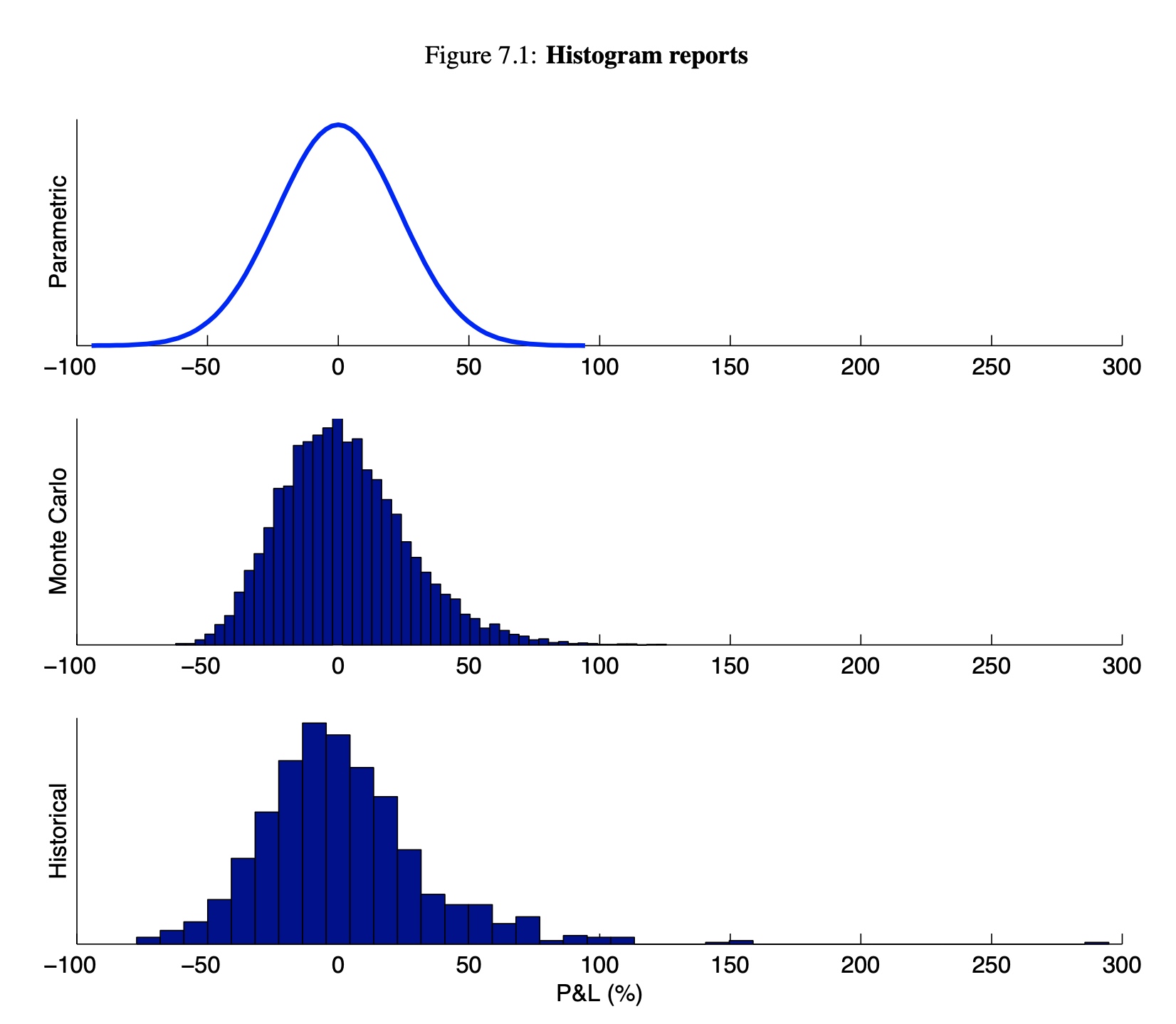
At a lower level of aggregation, we can use any of the risk measures described in Chapter 6 to describe particular features of the P&L distribution in more detail. For example, we can calculate the 95% VaR and expected shortfall from the distributions in Figure 7.1. Table 7.1 shows the results.
\[\begin{aligned} &\text { Table } 7.1: 95 \% \text { VaR and Expected Shortfall }\\ &\begin{array}{lcc} & \text { VaR } & \text { Expected Shortfall } \\ \hline \text { Parametric } & -39 \% & -49 \% \\ \text { Monte Carlo } & -34 \% & -40 \% \\ \text { Historical } & -42 \% & -53 \% \end{array} \end{aligned}\]How to choose between different methods
The comparison of results from different methods is useful to study the effect of our distributional assumptions, and estimate the potential magnitude of the error incurred by the use of a model. However, in practice, it is often necessary to select from the parametric, historical, and Monte Carlo methods to facilitate the flow of information and consistency of results throughout an organization.
The selection of the calculation method should depend on the specific portfolio and the choice of distribution of risk factor returns.
- If the portfolio consists mainly of linear positions and we choose to use a normal distribution of returns:
- choose the parametric method due to its speed and accuracy under those circumstances
- If the portfolio consists mainly of non-linear positions,
- then we need to use either Monte Carlo or historical simulation depending on the desired distribution of returns.
The selection between the normal and empirical distributions is usually done based on practical considerations rather than through statistical tests.
The main reason to use the empirical distribution is to assign greater likelihood to large returns which have a small probability of occurrence under the normal distribution. Problems associated with empirical distribution:
- Length of Time Periods: The first problem is the difficulty of selecting the historical period used to construct the distribution.
- In addition, the scarcity of historical data makes it difficult to extend the analysis horizon beyond a few days2.
Risk concentrations in specific groups of positions
When dealing with complex or large portfolios, we will often need finer detail in the analysis. We can use risk measures to “dissect” risk across different dimensions and identify the sources of portfolio risk.
This is useful to identify risk concentrations by business unit, asset class, country, currency, and maybe even all the way down to the trader or instrument level.
For example, we can create a VaR table, where we show the risk of every business unit across rows, and counterparties across columns.
These different choices of rows and columns are called “drilldown dimensions”.

The next section describes drilldowns in detail and explains how to calculate statistics in each of the buckets defined by a drilldown dimension.
Drilldowns
We refer to the categories in which you can slice the risk of a portfolio as “drilldown dimensions”.
Examples of drilldown dimensions are: position, portfolio, asset type, counterparty, currency, risk type (e.g., foreign exchange, interest rate, equity), and yield curve maturity buckets.
Drilldowns using simulation methods
To produce a drilldown report for any statistic, we have to simulate changes in the risk factors contained in each bucket while keeping the remaining risk factors constant.
Once we have the change in value for each scenario on each bucket, we can calculate risk statistics using the $\Delta V$ information per bucket. In the following example, we illustrate the calculation of $\Delta V$ per bucket for one scenario.
Drilldowns using parametric methods
Drilldowns using the parametric approach are based on delta equivalents rather than scenarios, that is, to calculate a risk statistic for each bucket, we set the delta equivalents falling outside the bucket equal to zero, and proceed to calculate the statistic as usual. This procedure is best explained with an example.
Up to this point, we have presented some of the most common and effective ways of presenting the risk information as well as the methods to break down the aggregate risk in different dimensions. We have also emphasized the importance of looking at risk in many different ways in order to reveal potential exposures or concentrations to groups of risk factors. In the following section, we present a case study that provides a practical application of the reporting concepts we have introduced.
Global Bank case study
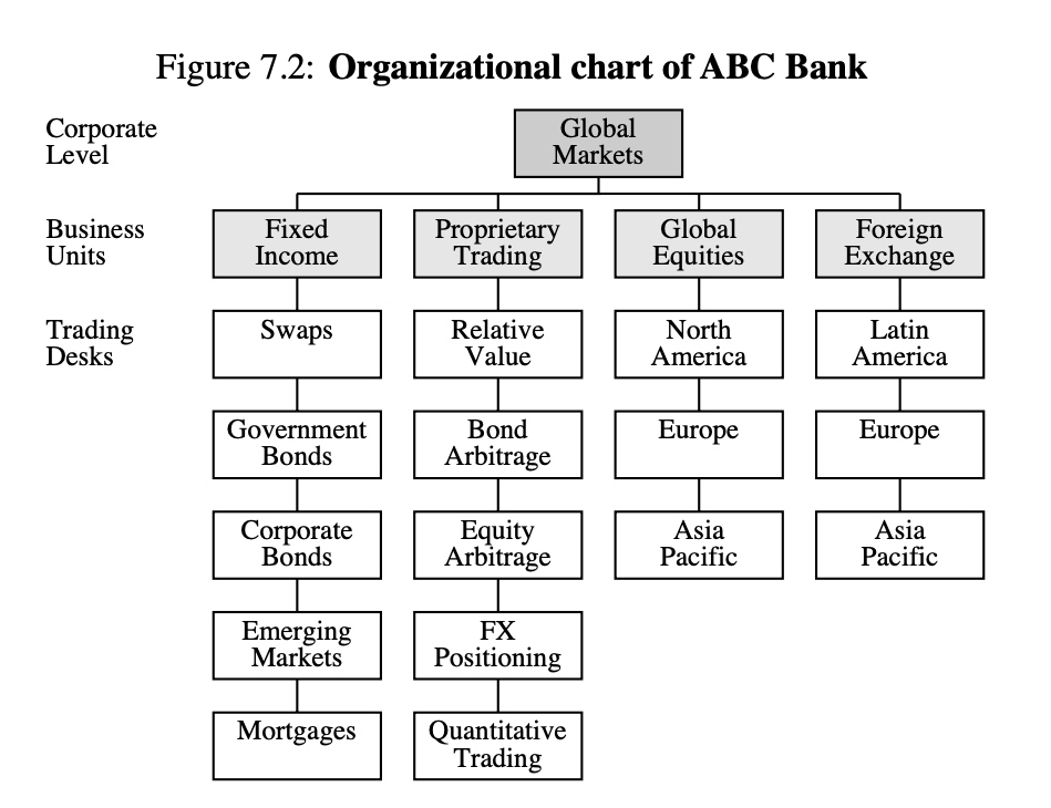
Risk reporting is one of the most important aspects of risk management. Effective risk reports help understand the nature of market risks arising from different business units, countries, positions, and risk factors in order to prevent or act effectively in crisis situations. This section presents the example of a fictitious bank, ABC, which is structured in three organizational levels: corporate level, business units, and trading desks. Figure 7.2 presents the organizational chart of ABC bank. The format and content of each risk report is designed to suit the needs of each organizational level.
Corporate Level At the corporate level, senior management needs a firmwide view of risk, and they will typically focus on market risk concentrations across business units as well as global stress test scenarios.
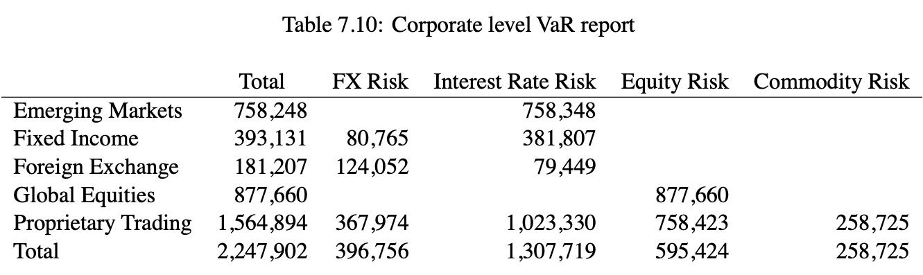
Table 7.10 reports VaR by business unit and risk type.
- We can see that the one-day 95% VaR is USD 2,247,902.
- Among the business units, proprietary trading has the highest VaR level (USD 1,564,894), mainly as a result of their interest rate and equity exposures.
- However, the equity exposures in proprietary trading offset exposures in global equities resulting in a low total equity risk for the bank (USD 595,424).
- Similarly, the interest rate exposures taken by the proprietary trading unit are offsetting exposures in the emerging markets, fixed income, and foreign exchange units.
- We can also observe that the foreign exchange unit has a high interest rate risk reflecting the existence of FX forwards, futures, and options in their inventory.
Business units Level Business units usually need to report risk by trading desk, showing more detail than the corporate reports. For example, a report at the business unit level might contain information by trading desk and country or currency. Table 7.11 reports VaR for the Foreign Exchange unit by trading desk and instrument type. For each instrument type the risk is reported by currency.
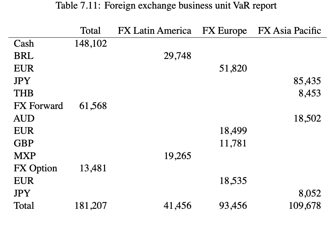
- We can see that most of ABC’s FX risk is in cash (USD 148,102) with the single largest exposure denominated in JPY (USD 85,435).
- Also note that the FX Europe trading desk creates a concentration in EUR across cash, FX forward, and FX option instruments which accounts for most of its USD 93,456 at risk.
Trading desk Level
At the trading desk level, risk information is presented at the most granular level. Trading desk reports might include detailed risk information by trader, position, and drilldowns such as yield curve positioning. Table 7.12 reports the VaR of the Government Bonds desk by trader and yield curve bucket.

- We can observe that Trader A is exposed only to fluctuations in the short end of the yield curve, while Trader C is well diversified across the entire term structure of interest rates.
- We can also see that trader B has a barbell exposure to interest rates in the intervals from six months to three years and fifteen years to thirty years.
- Note that the risk of the desk is diversified across the three traders.
- We can also see that the VaR of the Government Bonds desk (USD 122,522) is roughly one third of the VaR for the Fixed Income unit (USD 393,131).
Summary
This document provides an overview of the methodology currently used by RiskMetrics in our market risk management applications. Part I discusses the mathematical assumptions of the multivariate normal model and the empirical model for the distribution of risk factor returns, as well as the parametric and simulation methods used to characterize such distributions. In addition, Part I gives a description of stress testing methods to complement the statistical models. Part II illustrates the different pricing approaches and the assumptions made in order to cover a wide set of asset types. Finally, Part III explains how to calculate risk statistics using the methods in Part I in conjunction with the pricing functions of Part II. We conclude the document by showing how to create effective risk reports based on risk statistics.
The models, assumptions, and techniques described in this document lay a solid methodological foundation for market risk measurement upon which future improvements will undoubtedly be made. We hope to have provided a coherent framework for understanding and using risk modeling techniques.
Comments