Test Statistic
A test is based on a statistic, which estimates the parameter that appears in the hypotheses – Point estimate
Values of the estimate far from the parameter value in H0 give evidence against H0.
$H_a$ determines which direction will be counted as “far from the parameter value”.
Commonly, the test statistic has the form
$T=\frac{\text{estimate - hypothesized value}}{\text{standard deviation of the estimate} }$
One-Sample T Test: Test Statistic
Parameter $\mu$ with hypothesized value $\mu_0$
Estimate $\bar{X}$ with observed value $\bar{x}$, and estimated standard deviation $s/\sqrt{n}$
Test statistics
\[T=\frac{\bar{X}-\mu_0}{s/\sqrt{n}}\]with observed value
\[t=\frac{\bar{x}-\mu_0}{s/\sqrt{n}}\]State null and alternative hypothesis:
\[\begin{array}{r} \mu \neq \mu_{0} \\ H_{0}: \mu=\mu_{0} \quad v s . \quad H_{a}: \quad \mu>\mu_{0} \\ \mu<\mu_{0} \end{array}\]p-value equals, assuming $H_0$ holds
\[2P(T\geq \vert t \vert )\\ P(T\geq t )\\ P(T\leq t )\]Hypothesis Testing: Type I and Type II Errors
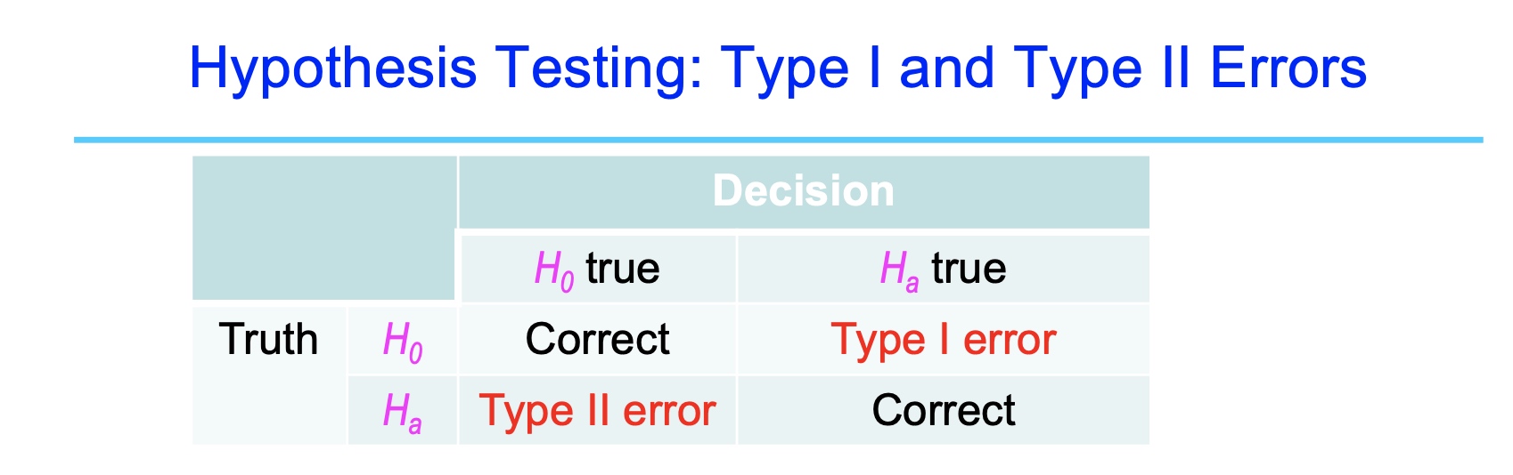
To limit the chance of a Type I Error to a chosen level α:
- referred to as significance level
- upper bound on Type I error
- commonly set at 5%
Reject $H_0$ when the p-value <= α
If so, we claim that the data support the alternative Ha at level α, or
– The data are statistically significant at level α
Relation between P-value and significance level α :
- Reject H0 if p-value <= α
- Do not reject H0 if p-value > α.
Two-Sample t-Test for Equal Means
Purpose: Test if two population means are equal
The two-sample t-test (Snedecor and Cochran, 1989) is used to determine if two population means are equal. A common application is to test if a new process or treatment is superior to a current process or treatment.
There are several variations on this test.
-
The data may either be paired or not paired. By paired, we mean that there is a one-to-one correspondence between the values in the two samples. That is, if X1, X2, …, Xn and Y1, Y2, … , Yn are the two samples, then Xi corresponds to Yi. For paired samples, the difference Xi - Yi is usually calculated. For unpaired samples, the sample sizes for the two samples may or may not be equal. The formulas for paired data are somewhat simpler than the formulas for unpaired data.
-
The variances of the two samples may be assumed to be equal or unequal. Equal variances yields somewhat simpler formulas, although with computers this is no longer a significant issue.
-
In some applications, you may want to adopt a new process or treatment only if it exceeds the current treatment by some threshold. In this case, we can state the null hypothesis in the form that the difference between the two populations means is equal to some constant μ1−μ2=d0 where the constant is the desired threshold.
Definition of Two-Sample t-test
The two-sample t-test for unpaired data is defined as:
\[\begin{array}{ll} \mathrm{H}_{0}: & \mu_{1}=\mu_{2} \\ \mathrm{H}_{\mathrm{a}}: & \mu_{1} \neq \mu_{2} \\ \text { Test Statistic: } & T=\frac{\bar{Y}_{1}-\bar{Y}_{2}}{\sqrt{s_{1}^{2} / N_{1}+s_{2}^{2} / N_{2}}} \end{array}\]where $N_1$ and $N_2$ are the sample sizes, $\bar{Y}_1$ and $\bar{Y}_2$ are the sample means, and $s_1^2$ and $s_2^2$ are the sample variances.
Significance Level: $\alpha$
Critical Region: Reject the null hypothesis that the two means are equal if
\[\vert T \vert > t_{1-\alpha/2,v}\]where $t_{1-\alpha/2,v}$ is the critical value of t-distribution with v degrees of freedom.
For the unequal variance case:
\[v=\frac{\left(s_{1}^{2} / N_{1}+s_{2}^{2} / N_{2}\right)^{2}}{\left(s_{1}^{2} / N_{1}\right)^{2} /\left(N_{1}-1\right)+\left(s_{2}^{2} / N_{2}\right)^{2} /\left(N_{2}-1\right)}\]For the equal variance case:
\[v=N_1 + N_2 -2\]Two-Sample t-Test Example
The following two-sample t-test was generated for the AUTO83B.DAT data set. The data set contains miles per gallon for U.S. cars (sample 1) and for Japanese cars (sample 2); the summary statistics for each sample are shown below.
SAMPLE 1
1
2
3
4
    NUMBER OF OBSERVATIONS      = 249
    MEAN                        =  20.14458
    STANDARD DEVIATION          =   6.41470
    STANDARD ERROR OF THE MEAN  =   0.40652
SAMPLE 2
1
2
3
4
    NUMBER OF OBSERVATIONS      = 79
    MEAN                        = 30.48101
    STANDARD DEVIATION          =  6.10771
    STANDARD ERROR OF THE MEAN  =  0.68717
We are testing the hypothesis that the population means are equal for the two samples. We assume that the variances for the two samples are equal.
\[\mathrm{H}_{0}: \quad \mu_{1}=\mu_{2}\] \[\mathrm{H}_{\mathrm{a}}: \quad \mu_{1} \neq \mu_{2}\]Test statistic: $T=-12.62059$
Pooled standard deviation: $\quad s_{p}=6.34260$
Degrees of freedom: $v=326$
significance level: $\alpha=0.05$
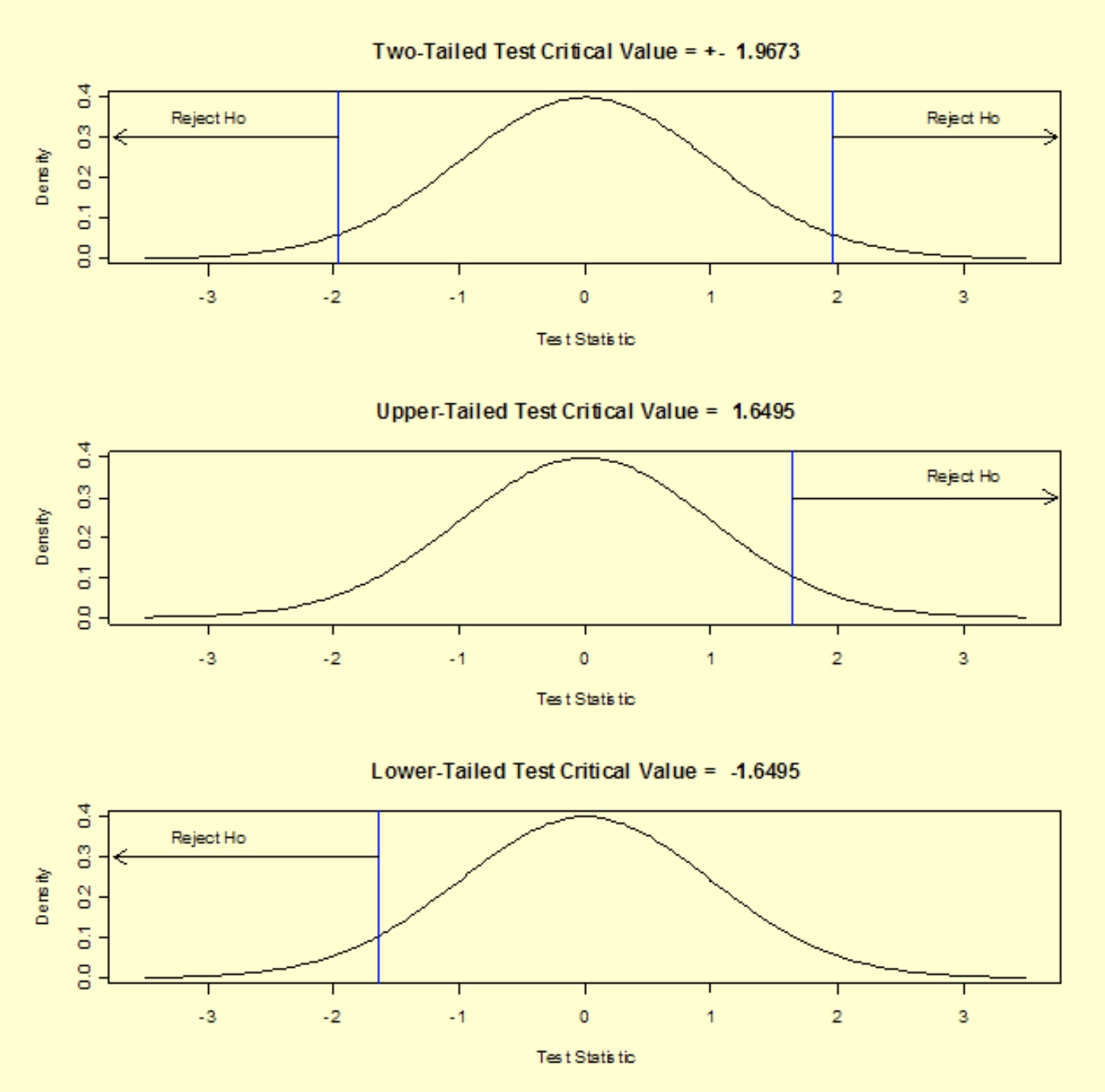
Critical value (upper tail): $t_{1-\alpha / 2, v}=1.9673$
Critical region: Reject $\mathrm{H}_{0}$ if $\vert T \vert >1.9673$
The absolute value of the test statistic for our example, 12.62059, is greater than the critical value of 1.9673, so we reject the null hypothesis and conclude that the two population means are different at the 0.05 significance level.
In general, there are three possible alternative hypotheses and rejection regions for the one-sample t-test:
\[\begin{array}{|l|l|} \hline \text { Alternative Hypothesis } & \text { Rejection Region } \\ \hline \mathrm{H}_{\mathrm{a}}: \mu_{1} \neq \mu_{2} & |T|>t_{1-\alpha / 2, v} \\ \hline \mathrm{H}_{\mathrm{a}}: \mu_{1}>\mu_{2} & T>t_{1-\alpha, v} \\ \hline \mathrm{H}_{\mathrm{a}}: \mu_{1}<\mu_{2} & T<t_{\alpha, v} \\ \hline \end{array}\]For our two-tailed t-test, the critical value is $t_{1-\alpha / 2, v} = 1.9673$, where α = 0.05 and ν = 326. If we were to perform an upper, one-tailed test, the critical value would be $t_{1-\alpha / 2, v} = 1.6495$. The rejection regions for three possible alternative hypotheses using our example data are shown below.
One way ANOVA
One-way ANOVA overview
In an analysis of variance, the variation in the response measurements is partitoined into components that correspond to different sources of variation.
The goal in this procedure is to split the total variation in the data into a portion due to random error and portions due to changes in the values of the independent variable(s).
The variance of n measurements is given by
\[s^2 = \frac{\sum_{i=1}^n (y_i - \bar{y})^2}{n-1} \, ,\]where $\bar{y}$ is the mean of the n measurements.
The numerator part is called the sum of squares of deviations from the mean, and the denominator is called the degrees of freedom.
The SS in a one-way ANOVA can be split into two components, called the “sum of squares of treatments” and “sum of squares of error”, abbreviated as SST and SSE, respectively.
Algebraically, this is expressed by
\[\begin{array}{ccccc} SS(Total) & = & SST & + & SSE \\ & & & & \\ \sum_{i=1}^k \sum_{j=1}^{n_i} (y_{ij} - \bar{y}_{\huge{\cdot \cdot}})^2 & = & \sum_{i=1}^k n_i (\bar{y}_{i \huge{\cdot}} - \bar{y}_{\huge{\cdot \cdot}})^2 & + & \sum_{i=1}^k \sum_{j=1}^{n_i} (y_{ij} - \bar{y}_{i \huge{\cdot}})^2 \, , \end{array}\]where k is the number of treatments and the bar over the $y_{\huge{\cdot \cdot}}$ denotes the “grand” or “overall” mean. Each $n_i$ is the number of observations for treatment i. The total number of observations is N (the sum of the $n_i$).
The one-way ANOVA model and assumptions
The mathematical model that describes the relationship between the response and treatment for the one-way ANOVA is given by
\[Y_{ij} = \mu + \tau_i + \epsilon_{ij} \, ,\]where $Y_{ij}$ represents the j-th observation (j=1,2,…,$n_i$) on the i-th treatment (i=1,2,…,k levels). So, Y23 represents the third observation using level 2 of the factor. μ is the common effect for the whole experiment, τi represents the i-th treatment effect, and ϵij represents the random error present in the j-th observation on the i-th treatment.
Fixed effects model
The errors ϵij are assumed to be normally and independently (NID) distributed, with mean zero and variance $\sigma^2_{\varepsilon}$. $\mu$ is always a fixed parameter, and $\tau_1, \, \tau_2, \, \ldots, \, \tau_k$ are considered to be fixed parameters if the levels of the treatment are fixed and not a random sample from a population of possible levels. It is also assumed that $\mu$ is chosen so that
\[\sum \tau_i = 0 \, , \,\,\,\,\, i = 1, \, \ldots, \, k\]holds. This is the fixed effects model.
Random effects mode
If the k levels of treatment are chosen at random, the model equation remains the same. However, now the $\tau_i$ values are random variables assumed to be $NID(0, \sigma_{\tau})$. This is the random effects model.
Whether the levels are fixed or random depends on how these levels are chosen in a given experiment.
The ANOVA table and tests of hypotheses about means
Sums of Squares help us compute the variance estimates displayed in ANOVA Tables.
The sums of squares SST and SSE previously computed for the one-way ANOVA are used to form two mean squares, one for treatments and the second for error. These mean squares are denoted by MST and MSE, respectively. These are typically displayed in a tabular form, known as an ANOVA Table. The ANOVA table also shows the statistics used to test hypotheses about the population means.
When the null hypothesis of equal means is true, the two mean squares estimate the same quantity (error variance), and should be of approximately equal magnitude. In other words, their ratio should be close to 1. If the null hypothesis is false, MST should be larger than MSE.
Let $N=\sum n_i$. Then, the degrees of freedom for treatment are
\[DFT = k - 1 \, ,\]and the degrees of freedom for error are
\[DFE = N - k \, .\]The corresponding mean squares are:
\[MST=SST/DFT\] \[MSE=SSE/DFE\]F-test
The test statistic, used in testing the equality of treatment means is: F=MST/MSE.
The critical value is the tabular value of the F distribution, based on the chosen $\alpha$ level and the degrees of freedom DFT and DFE.
The calculations are displayed in an ANOVA table, as follows:
\[\begin{array}{ccccc} \hline \text { Source } & \text { SS } & \text { DF } & \text { MS } & \text { F } \\ \hline & & & & \\ \text { Treatments } & S S T & k-1 & S S T /(k-1) & M S T / M S E \\ \text { Error } & S S E & N-k & S S E /(N-k) & \\ \hline \text { Total (corrected) } & S S & N-1 & & \\ \hline \end{array}\]The word “source” stands for source of variation. Some authors prefer to use “between” and “within” instead of “treatments” and “error”, respectively.
ANOVA Table Example
The data below resulted from measuring the difference in resistance resulting from subjecting identical resistors to three different temperatures for a period of 24 hours. The sample size of each group was 5. In the language of design of experiments, we have an experiment in which each of three treatments was replicated 5 times.
\[\begin{aligned} &\begin{array}{lccc} \hline &\text { Level 1 } & \text { Level 2 } & \text { Level 3 } \\ &\hline 6.9 & 8.3 & 8.0 \\ &5.4 & 6.8 & 10.5 \\ &5.8 & 7.8 & 8.1 \\ &4.6 & 9.2 & 6.9 \\ &4.0 & 6.5 & 9.3 \\ \hline \text{mean} &5.34 & 7.72 & 8.56 \\ \hline \end{array} \end{aligned}\]The resulting ANOVA table is
\[\begin{array}{ccccc} \hline \text { Source } & \text { SS } & \text { DF } & \text { MS } & \text { F } \\ \hline \text { Treatments } & 27.897 & 2 & 13.949 & 9.59 \\ \text { Error } & 17.452 & 12 & 1.454 & \\ \hline & & & & \\ \hline \text { Total (corrected) } & 45.349 & 14 & & \\ \text { Correction Factor } & 779.041 & 1 & & \end{array}\]The test statistic is the F value of 9.59. Using an α of 0.05, we have $F_{0.05; \, 2, \, 12}= 3.89$.
Since the test statistic is much larger than the critical value, we reject the null hypothesis of equal population means and conclude that there is a (statistically) significant difference among the population means. The p-value for 9.59 is 0.00325, so the test statistic is significant at that level.
The populations here are resistor readings while operating under the three different temperatures. What we do not know at this point is whether the three means are all different or which of the three means is different from the other two, and by how much.
There are several techniques we might use to further analyze the differences. These are:
- constructing confidence intervals around the difference of two means,
- estimating combinations of factor levels with confidence bounds
- multiple comparisons of combinations of factor levels tested simultaneously.
Confidence intervals for the difference of treatment means
This page shows how to construct a confidence interval around (μi−μj) for the one-way ANOVA by continuing the example shown on a previous page.
The formula for a 100(1−α) % confidence interval for the difference between two treatment means is:
\[(\hat{\mu_i} - \hat{\mu_j}) \pm t_{1-\alpha/2, \, N-k} \,\,\sqrt{\hat{\sigma}^2_\epsilon \left( \frac{1}{n_i}+\frac{1}{n_j}\right)} \, ,\]where $\hat{\sigma}_\epsilon^2 = MSE$.
For the example, we have the following quantities for the formula
- $\bar{y}_3=8.56$
- $\bar{y}_1=5.34$
- $\sqrt{1.454(1/5 + 1/5)} = 0.763$
- $t_{0.975, \, 12} = 2.179$
Substituting these values yields (8.56 - 5.34) ± 2.179(0.763) or 3.22 ± 1.663.
That is, the confidence interval is (1.557, 4.883).
A 95 % confidence interval for μ3−μ2 is: (-1.787, 3.467).
A 95 % confidence interval for μ2−μ1 is: (-0.247, 5.007).
Application: Employee Performance Study
Data set:
- 150 managers: 88 internal and 62 external
- Manager Rating is an evaluation score of the employee in their current job, indicating the “value” of the employee to the firm
- Origin is a categorical variable that identifies the managers as either External or Internal to indicate from where they were hired
- Salary is the starting salary of the employee when they were hired. It indicates what sort of job the person was initially hired to do. In the context of this example, it does not measure how well they did that job. That’s measured by the rating variable.
Two Sample Comparison: Manager Rating vs Origin
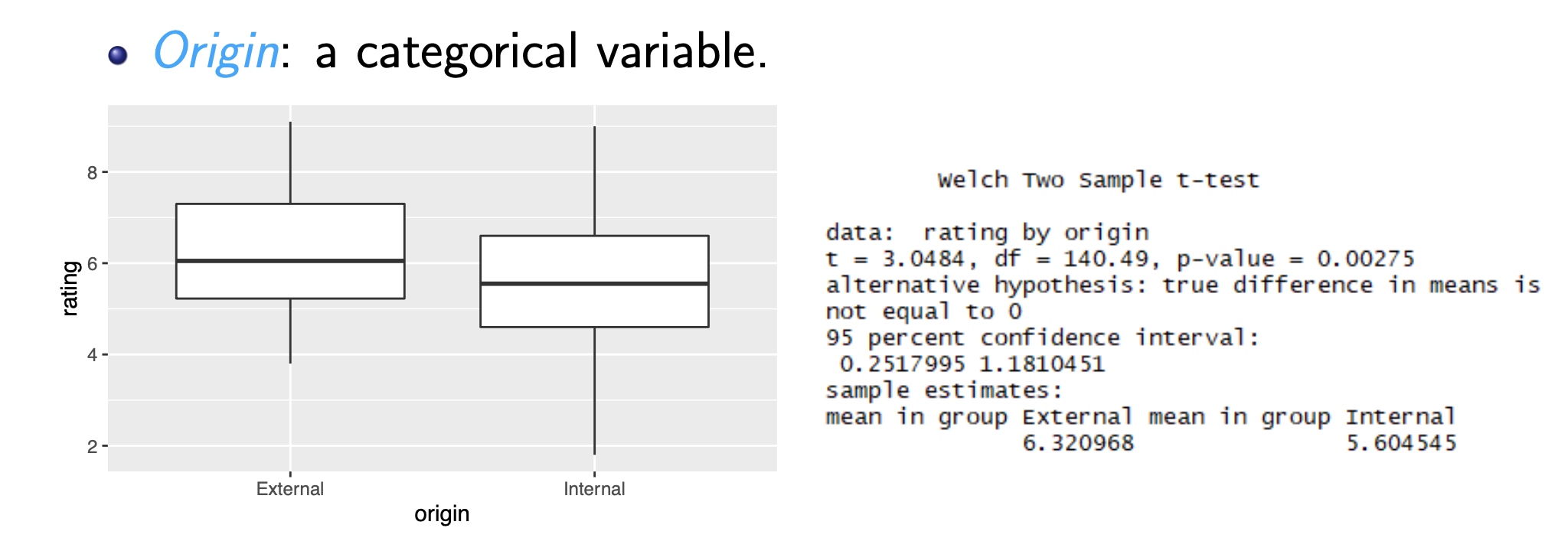
We can recognize a significant difference between the means via two-sample t-test.
One-way ANOVA
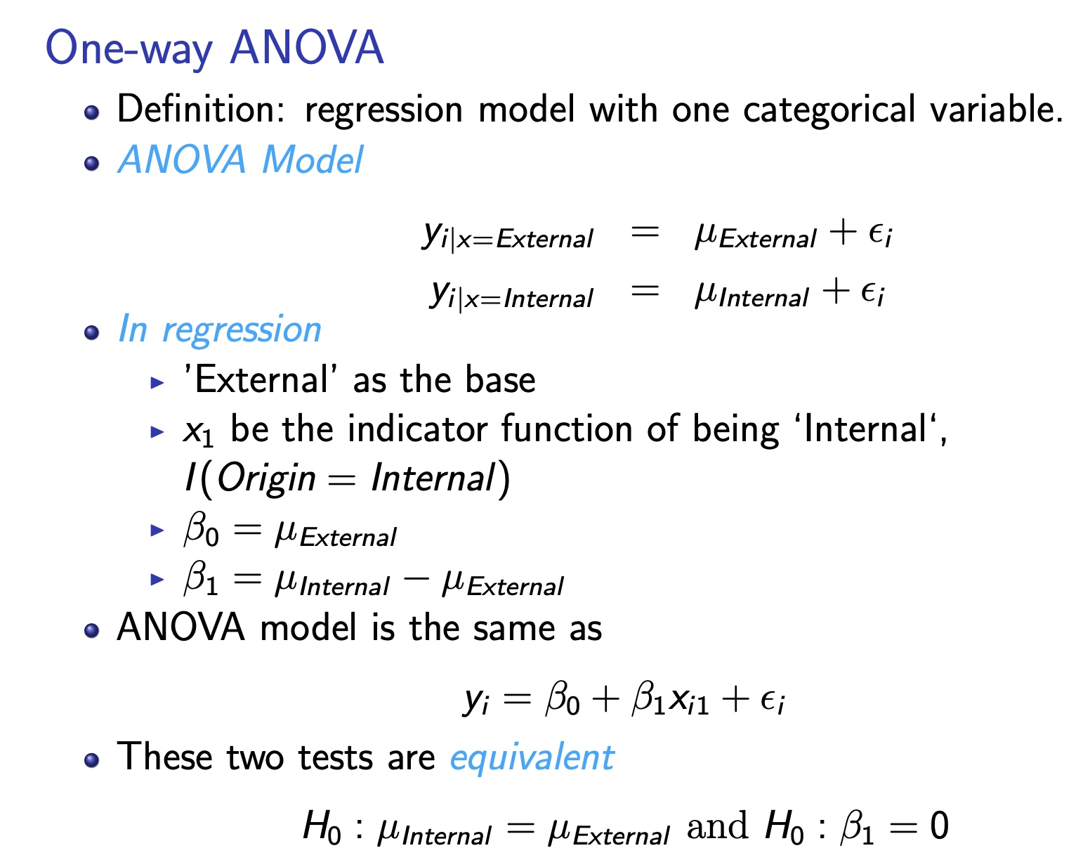
Regress Manager Rating on Origin:
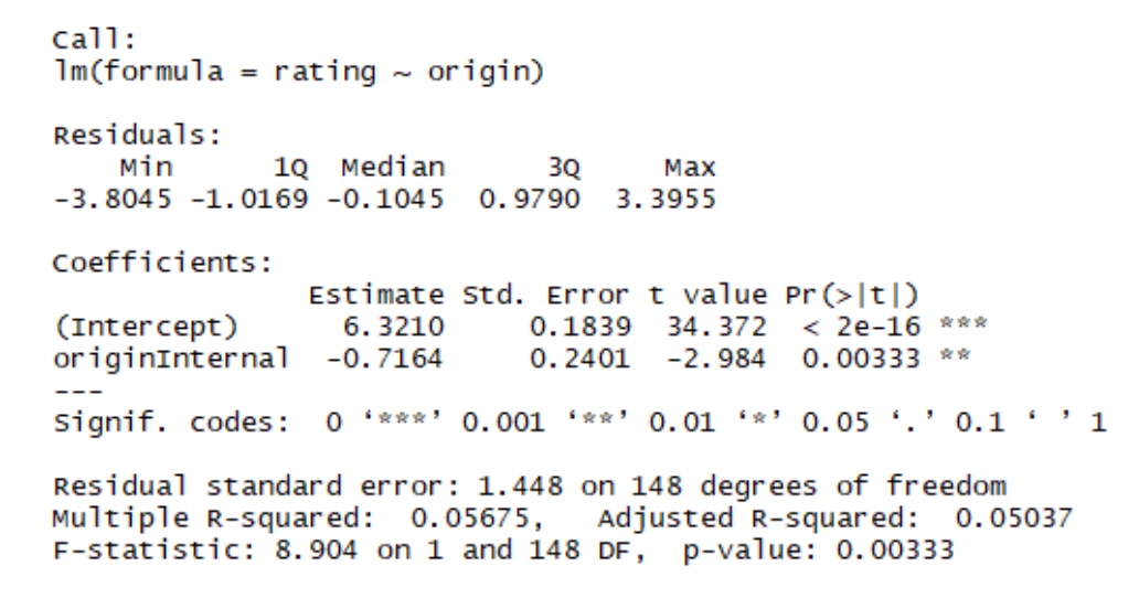
- The difference in the rating (-0.72) between internal and external managers is significant since the p-value = .003 < .05.
- In terms of regression, Origin explains significant variation in Manager Rating.
- Before we claim that the external candidate should be hired, is there a possible confounding variable, another explanation for the difference in rating?
- Let’s explore the relationship between Manager Rating and Salary.
Scatterplot of Manager Rating vs. Salary
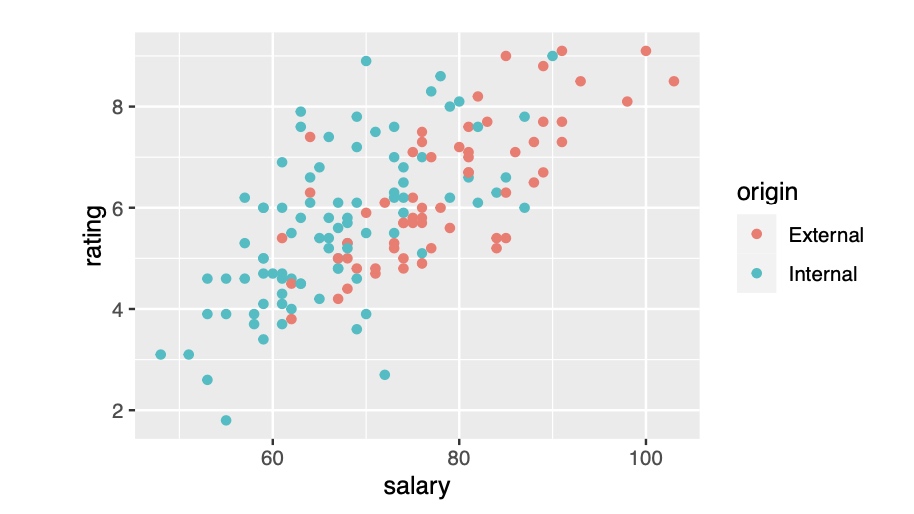
- (a) Salary is correlated with Manager Rating, and (b) that external managers were hired at higher salaries
- This combination indicates confounding: not only are we comparing internal vs. external managers; we are comparing internal managers hired into lower salary jobs with external managers placed into higher salary jobs.
- Easy fix: compare only those whose starting salary near $80K. But that leaves too few data points for a reasonable comparison.
Separate Regressions of Manager Rating on Salary
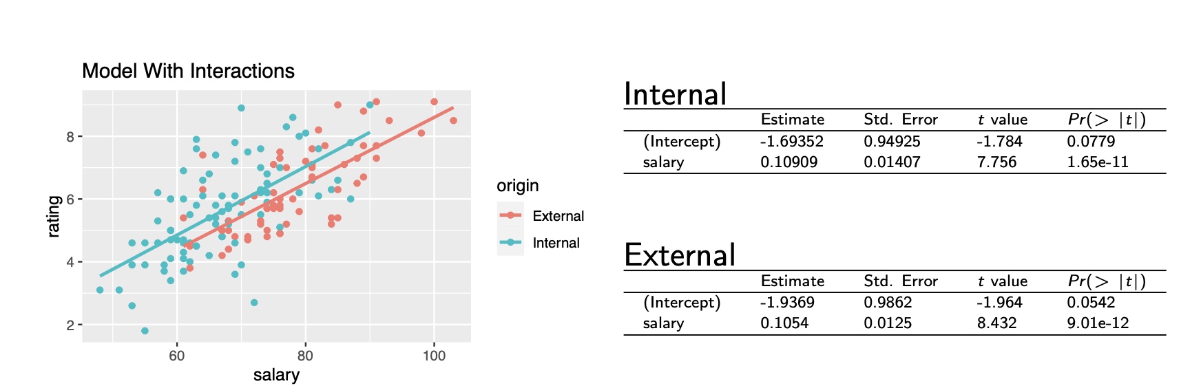
- Based on the regression, at any given salary, internal managers is expected to get higher average ratings!
- In regression, confounding is a form of collinearity.
- Salary is related to Origin which was the variable used to explain Rating.
- With Salary added, the effect of Origin changes sign. Now internal managers look better.
Are the Two Fits Significantly Different?
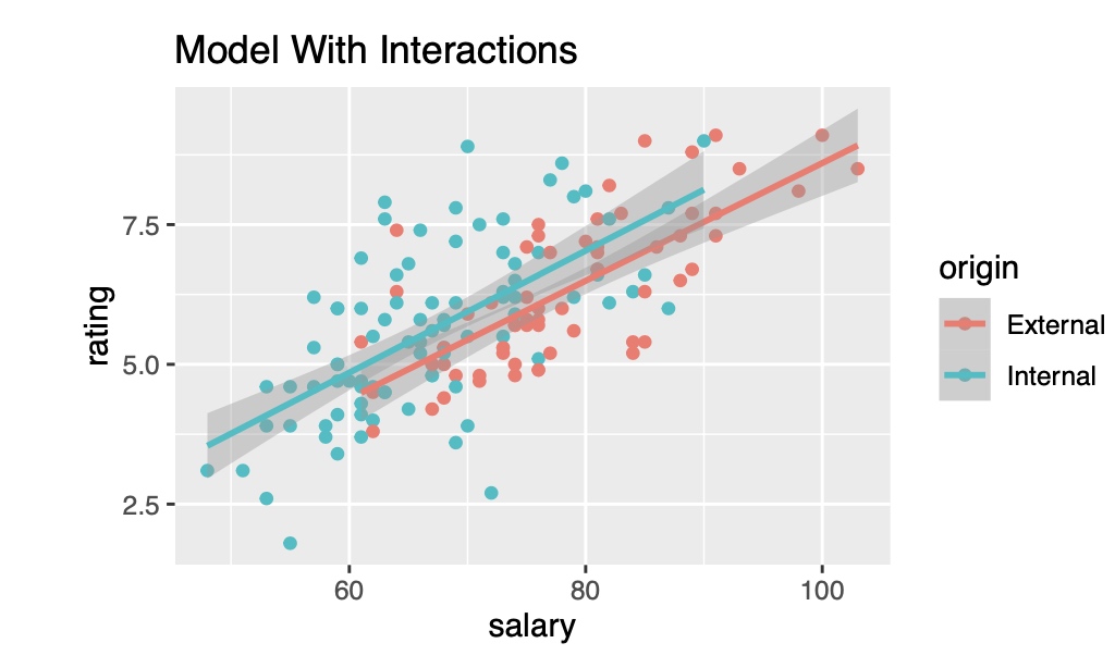
- The two confidence bands overlap, which make the comparison indecisive.
- A more powerful idea is to combine these two separate simple regressions into one multiple regression that will allow us to compare these fits.
Regress Manager Rating on both Salary and Origin
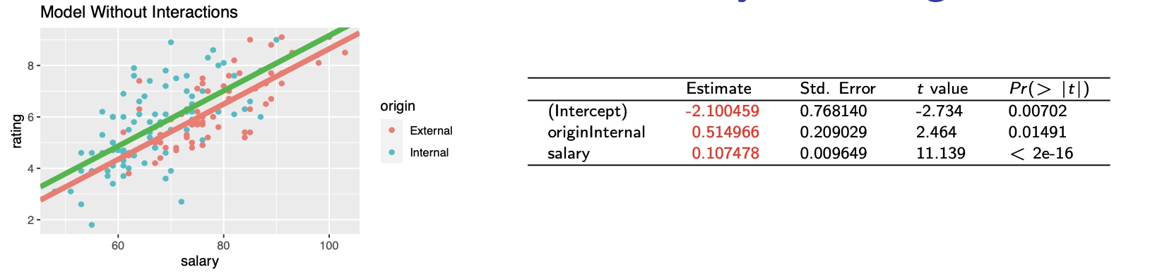
- x1 dummy variable of being ’Internal’, I(Origin = Internal)
- Notice that we only require one dummy variable to distinguish internal from external managers.
- This enables two parallel lines for two kinds of managers.
- If Origin = External, Manager Rating = -2.100459 + 0.107478 Salary
- If Origin = Internal, Manager Rating = -2.100459 + 0.107478 Salary + 0.514966
- The coefficient of the dummy variable is the difference between the intercepts.
- The difference between the intercepts is significantly different from 0, since 0.0149, the p-value for Origin[Internal], is less than 0.05.
- Thus, if we assume the slopes are equal, a model using a categorical predictor implies that controlling for initial salary, internal managers rate significantly higher.
- How can we check the assumption that the slopes are parallel?
Model with Interaction: Different Slopes
An interaction between a dummy variable $I_k$ and a numerical variable $x_i$ measures the difference between the slopes of the numerical variable in the two groups:
\[X_i * I_k\]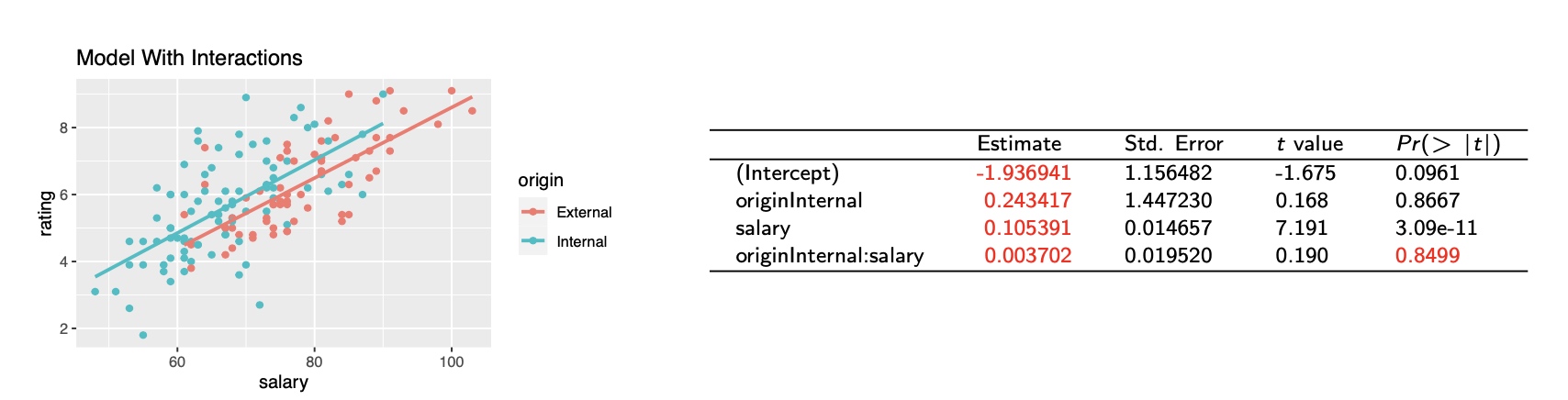
Interaction variable – product of the dummy variable and Salary:
\[\begin{aligned} \text { originlnternal:salary } &=\text { salary } & & \text { if Origin } &=\text { Internal } \\ &=0 & & \text { if Origin }=\text { External } \end{aligned}\]- If Origin = External:
- Manager Rating = -1.94 + 0.11 Salary
- If Origin = Internal:
- Manager Rating = (-1.94+0.24) + (0.11+0.0037) Salary= -1.69 + 0.11 Salary
- These equations match the simple regressions fit to the two groups separately. The interaction is not significant because its p-value is large.
Principle of Marginality
- Leave main effects in the model (here Salary and Origin) whenever an interaction that uses them is present in the fitted model. If the interaction is not statistically significant, remove the interaction from the model.
- Origin became insignificant when Salary∗Origin was added, which is due to collinearity.
- The assumption of equal error variance should also be checked by comparing box-plots of the residuals grouped by the levels of the categorical variable.

Summary of this example
- Categorical variables model the differences between groups using regression, while taking account of other variables.
- In a model with a categorical variable, the coefficients of the categorical terms indicate differences between parallel lines.
- In a model that includes interactions, the coefficients of the interaction measure the differences in the slopes between the groups.
- Significant categorical variable ⇒ different intercepts
- Significant interaction ⇒ different slopes
Statistical Significance and Practical Significance
When drawing conclusions from a hypothesis test, it is important to keep in mind the difference between Statistical and Practical Significance.
- Statistical Significance : We can be sure that !” is false i.e. the difference from the hypothesized value is too large to be attributed to chance. Statistics can answer this question.
- Practical Significance : Is the difference large enough that in practice we care? Statistics can not answer this one!
Comments