Machine Learning Part 1： Basics

All of this series is mainly based on the Machine Learning course given by Andrew Ng, which is hosted on cousera.org.

Introduction

What is Machine Learning?

Two definitions of Machine Learning are offered. Arthur Samuel described it as: “the field of study that gives computers the ability to learn without being explicitly programmed.” This is an older, informal definition.

Tom Mitchell provides a more modern definition: “A computer program is said to learn from experience E with respect to some class of tasks T and performance measure P, if its performance at tasks in T, as measured by P, improves with experience E.”

Example: playing checkers.

E = the experience of playing many games of checkers

T = the task of playing checkers.

P = the probability that the program will win the next game.

In general, any machine learning problem can be assigned to one of two broad classifications:

Supervised learning and Unsupervised learning.

Supervised Learning

In supervised learning, we are given a data set and already know what our correct output should look like, having the idea that there is a relationship between the input and the output.

Supervised learning problems are categorized into “regression” and “classification” problems. In a regression problem, we are trying to predict results within a continuous output, meaning that we are trying to map input variables to some continuous function. In a classification problem, we are instead trying to predict results in a discrete output. In other words, we are trying to map input variables into discrete categories.

Example 1:

Given data about the size of houses on the real estate market, try to predict their price. Price as a function of size is a continuous output, so this is a regression problem.

We could turn this example into a classification problem by instead making our output about whether the house “sells for more or less than the asking price.” Here we are classifying the houses based on price into two discrete categories.

Example 2:

(a) Regression - Given a picture of a person, we have to predict their age on the basis of the given picture

(b) Classification - Given a patient with a tumor, we have to predict whether the tumor is malignant or benign.

Unsupervised Learning

Unsupervised learning allows us to approach problems with little or no idea what our results should look like. We can derive structure from data where we don’t necessarily know the effect of the variables.

We can derive this structure by clustering the data based on relationships among the variables in the data.

With unsupervised learning there is no feedback based on the prediction results.

Example:

Clustering: Take a collection of 1,000,000 different genes, and find a way to automatically group these genes into groups that are somehow similar or related by different variables, such as lifespan, location, roles, and so on.

Non-clustering: The “Cocktail Party Algorithm”, allows you to find structure in a chaotic environment. (i.e. identifying individual voices and music from a mesh of sounds at a cocktail party).

Model and Cost Function

Model Representation

To establish notation for future use, we’ll use $x^{(i)}$ to denote the “input” variables (living area in this example), also called input features, and $y^{(i)}$ to denote the “output” or target variable that we are trying to predict (price). A pair $(x^{(i)} , y^{(i)} )$ is called a training example, and the dataset that we’ll be using to learn—a list of m training examples $(x^{(i)} , y^{(i)} )$; i=1,…,m—is called a training set. Note that the superscript “(i)” in the notation is simply an index into the training set, and has nothing to do with exponentiation. We will also use X to denote the space of input values, and Y to denote the space of output values. In this example, X = Y = $\mathcal{R}$.

To describe the supervised learning problem slightly more formally, our goal is, given a training set, to learn a function h : X → Y so that h(x) is a “good” predictor for the corresponding value of y. For historical reasons, this function h is called a hypothesis. Seen pictorially, the process is therefore like this:

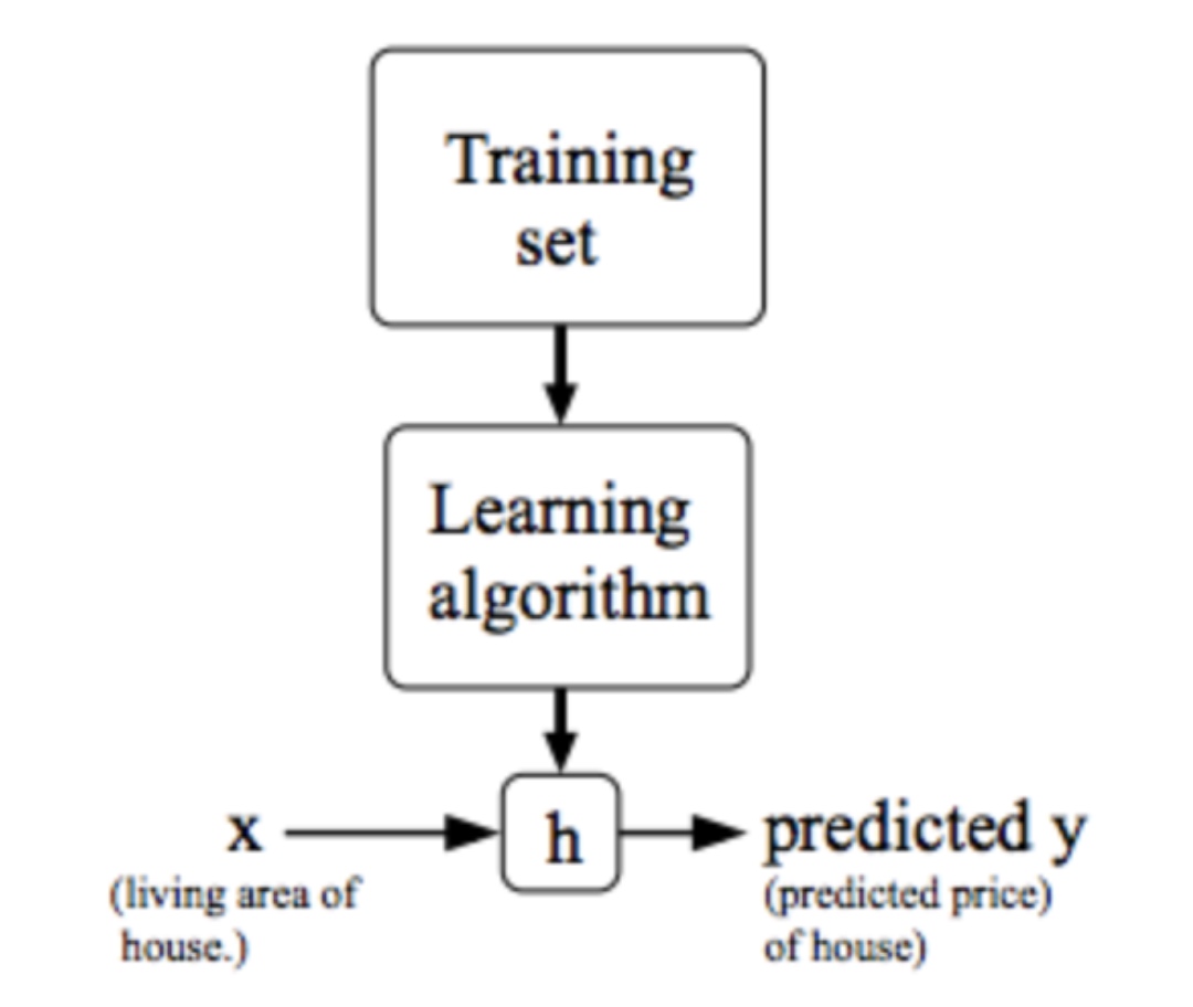
When the target variable that we’re trying to predict is continuous, such as in our housing example, we call the learning problem a regression problem. When y can take on only a small number of discrete values (such as if, given the living area, we wanted to predict if a dwelling is a house or an apartment, say), we call it a classification problem.

$h_\theta(x)=\theta_0+\theta_1*x$

Cost Function

We can measure the accuracy of our hypothesis function by using a cost function. This takes an average difference (actually a fancier version of an average) of all the results of the hypothesis with inputs from x’s and the actual output y’s.

\[J\left(\theta_{0}, \theta_{1}\right)=\frac{1}{2 m} \sum_{i=1}^{m}\left(\hat{y}_{i}-y_{i}\right)^{2}=\frac{1}{2 m} \sum_{i=1}^{m}\left(h_{\theta}\left(x_{i}\right)-y_{i}\right)^{2}\]

To break it apart, it is $\frac{1}{2}\bar{x}$ where $\bar{x}$ is the mean of the squares of $h_{\theta}\left(x_{i}\right)-y_{i}$ , or the difference between the predicted value and the actual value.

This function is otherwise called the “Squared error function”, or “Mean squared error”. The mean is halved $\left(\frac{1}{2}\right)$ as a convenience for the computation of the gradient descent, as the derivative term of the square function will cancel out the $\frac{1}{2}$ term. The following image summarizes what the cost function does:

\[\min_{\theta } ~~J(\theta )=\frac{1}{2 m} \sum_{i=1}^{m}\left(\hat{y}_{i}-y_{i}\right)^{2}=\frac{1}{2 m} \sum_{i=1}^{m}\left(h_{\theta}\left(x_{i}\right)-y_{i}\right)^{2}\]

Parameter Learning

Gradient Descent

So we have our hypothesis function and we have a way of measuring how well it fits into the data. Now we need to estimate the parameters in the hypothesis function. That’s where gradient descent comes in.

Imagine that we graph our hypothesis function based on its fields $\theta_0$ and $\theta_1$ (actually we are graphing the cost function as a function of the parameter estimates). We are not graphing x and y itself, but the parameter range of our hypothesis function and the cost resulting from selecting a particular set of parameters.

We put $\theta_0$ on the x axis and $\theta_1$ on the y axis, with the cost function on the vertical z axis. The points on our graph will be the result of the cost function using our hypothesis with those specific theta parameters. The graph below depicts such a setup.

We will know that we have succeeded when our cost function is at the very bottom of the pits in our graph, i.e. when its value is the minimum. The red arrows show the minimum points in the graph.

The gradient descent algorithm is:

\[\begin{array}{ll}{\text { repeat until convergence }\{ } \\ {\qquad \theta_{j} :=\theta_{j}-\alpha \frac{\partial}{\partial \theta_{j}} J\left(\theta_{0}, \theta_{1}\right) \quad \text { (simultaneously update $\theta_0$ and $\theta_1$ }} \\ { \}}\end{array}\]

At each iteration j, one should simultaneously update the parameters $\theta_1, \theta_2,…,\theta_n$. Updating a specific parameter prior to calculating another one on the $j^{(th)}$ iteration would yield to a wrong implementation.

$\alpha := learning~ rate$. On a side note, we should adjust our parameter \alphaα to ensure that the gradient descent algorithm converges in a reasonable time. Failure to converge or too much time to obtain the minimum value imply that our step size is wrong.

How does gradient descent converge with a fixed step size $\alpha$?

The intuition behind the convergence is that $\frac{d}{d\theta_1} J(\theta_1)$ approaches 0 as we approach the bottom of our convex function. At the minimum, the derivative will always be 0 and thus we get: $\theta_{1} :=\theta_{1}-\alpha * 0$

Gradient Descent for Linear Regression

For the cost function:

\[~~J(\theta )=\frac{1}{2 m} \sum_{i=1}^{m}\left(\hat{y}_{i}-y_{i}\right)^{2}=\frac{1}{2 m} \sum_{i=1}^{m}\left(h_{\theta}\left(x_{i}\right)-y_{i}\right)^{2}\]

Gradient Descent Algorithm

\[\begin{array}{l}{\text { repeat until convergence }\{ } \\ {\qquad \begin{array}{l}{\theta_{0} :=\theta_{0}-\alpha \frac{1}{m} \sum_{i=1}^{m}\left(h_{\theta}\left(x^{(i)}\right)-y^{(i)}\right)} \\ {\theta_{1} :=\theta_{1}-\alpha \frac{1}{m} \sum_{i=1}^{m}\left(h_{\theta}\left(x^{(i)}\right)-y^{(i)}\right) \cdot x^{(i)}}\end{array}}\end{array}\]

This method looks at every example in the entire training set on every step, and is called batch gradient descent. Note that, while gradient descent can be susceptible to local minima in general, the optimization problem we have posed here for linear regression has only one global, and no other local, optima; thus gradient descent always converges (assuming the learning rate α is not too large) to the global minimum. Indeed, J is a convex quadratic function.

Linear Algebra Review

Matrix

% The ; denotes we are going back to a new row.
A = [1, 2, 3; 4, 5, 6; 7, 8, 9; 10, 11, 12]

% Initialize a vector
v = [1;2;3]

% Get the dimension of the matrix A where m = rows and n = columns
[m,n] = size(A)

% You could also store it this way
dim_A = size(A)

% Get the dimension of the vector v
dim_v = size(v)

% Now let's index into the 2nd row 3rd column of matrix A
A_23 = A(2,3)

% Initialize matrix A and B
A = [1, 2, 4; 5, 3, 2]
B = [1, 3, 4; 1, 1, 1]

% Initialize constant s
s = 2

% See how element-wise addition works
add_AB = A + B

% See how element-wise subtraction works
sub_AB = A - B

% See how scalar multiplication works
mult_As = A * s

% Divide A by s
div_As = A / s

% What happens if we have a Matrix + scalar?
add_As = A + s

\[\left[\begin{array}{ll}{a} & {b} \\ {c} & {d} \\ {e} & {f}\end{array}\right] *\left[\begin{array}{l}{x} \\ {y}\end{array}\right]=\left[\begin{array}{l}{a * x+b * y} \\ {c * x+d * y} \\ {e * x+f * y}\end{array}\right]\]

% Initialize matrix A
A = [1, 2, 3; 4, 5, 6;7, 8, 9]

% Initialize vector v
v = [1; 1; 1]

% Multiply A * v
Av = A * v

An m x n matrix multiplied by an n x o matrix results in an m x o matrix. In the above example, a 3 x 2 matrix times a 2 x 2 matrix resulted in a 3 x 2 matrix. To multiply two matrices, the number of columns of the first matrix must equal the number of rows of the second matrix.

For example:

% Initialize a 3 by 2 matrix
A = [1, 2; 3, 4;5, 6]

% Initialize a 2 by 1 matrix
B = [1; 2]

% We expect a resulting matrix of (3 by 2)*(2 by 1) = (3 by 1)
mult_AB = A*B

% Make sure you understand why we got that result

Matrix Multiplication Properties

• Matrices are not commutative: A∗B≠B∗A
• Matrices are associative: (A∗B)∗C=A∗(B∗C)

% Initialize random matrices A and B
A = [1,2;4,5]
B = [1,1;0,2]

% Initialize a 2 by 2 identity matrix
I = eye(2)

% The above notation is the same as I = [1,0;0,1]

% What happens when we multiply I*A ?
IA = I*A

% How about A*I ?
AI = A*I

% Compute A*B
AB = A*B

% Is it equal to B*A?
BA = B*A

% Note that IA = AI but AB != BA

• Inverse of matrix A
• Transpose of A

Ainv=inv(A)
Atrans=transpose(A)
%Alternatively
Atrans2=A'

Multiple Linear regression

Linear regression with multiple variables is also known as “multivariate linear regression”.

We now introduce notation for equations where we can have any number of input variables.

\[\begin{aligned} x_{j}^{(i)} &=\text { value of feature } j \text { in the } i^{\text {th}} \text {training example } \\ x^{(i)} &=\text { the input (features) of the } i^{\text {th}} \text {training example } \\ m &=\text { the number of training examples } \\ n &=\text { the number of features } \end{aligned}\]

The multivariable form of the hypothesis function accommodating these multiple features is as follows:

$h_{\theta}(x)=\theta_{0}+\theta_{1} x_{1}+\theta_{2} x_{2}+\theta_{3} x_{3}+\cdots+\theta_{n} x_{n}$

Using the definition of matrix multiplication, our multivariable hypothesis function can be concisely represented as:

$h_{\theta}(x)=\theta^Tx$

Remark: Note that for convenience reasons in this course we assume $x_{0}^{(i)}=1 \text { for }(i \in 1, \ldots, m)$. This allows us to do matrix operations with theta and x. Hence making the two vectors $\theta$ and $x^{(i)}$ match each other element-wise (that is, have the same number of elements: n+1).]

Gradient Descent for Multiple Variables

repeat until convergence:

\[\begin{array}{l}{\theta_{0} :=\theta_{0}-\alpha \frac{1}{m} \sum_{i=1}^{m}\left(h_{\theta}\left(x^{(i)}\right)-y^{(i)}\right) x_{0}^{(i)}} \\ {\theta_{1} :=\theta_{1}-\alpha \frac{1}{m} \sum_{i=1}^{m}\left(h_{\theta}\left(x^{(i)}\right)-y^{(i)}\right) x_{1}^{(i)}} \\ {\theta_{2} :=\theta_{2}-\alpha \frac{1}{m} \sum_{i=1}^{m}\left(h_{\theta}\left(x^{(i)}\right)-y^{(i)}\right) x_{2}^{(i)}}\end{array} \\...\]

In other words:

\[\begin{array}{l}{\text { repeat until convergence: } } \\ {\theta_{j} :=\theta_{j}-\alpha \frac{1}{m} \sum_{i=1}^{m}\left(h_{\theta}\left(x^{(i)}\right)-y^{(i)}\right) \cdot x_{j}^{(i)} \quad \text { for } j :=0 \ldots n}\end{array}\]

$x_{0}^{(i)}=1, \forall i$

Vectorization

Use the built in functions to solve the calculation. Try not to implement the loop by ourselves.

For example, in the gradient descent method, we need to calculate simultaneously:

\[\begin{array}{l}{\text { repeat until convergence: } } \\ {\theta_{j} :=\theta_{j}-\alpha \frac{1}{m} \sum_{i=1}^{m}\left(h_{\theta}\left(x^{(i)}\right)-y^{(i)}\right) \cdot x_{j}^{(i)} \quad \text { for } j :=0 \ldots n}\end{array}\]

In fact, this is equivalent to:

$\theta_{new}=\theta-\frac{\alpha}{m}X^T(X\theta-y)$

Practice 1: Feature Scaling and Mean normalization

We can speed up gradient descent by having each of our input values in roughly the same range. This is because θ will descend quickly on small ranges and slowly on large ranges, and so will oscillate inefficiently down to the optimum when the variables are very uneven.

The way to prevent this is to modify the ranges of our input variables so that they are all roughly the same. Ideally:

$-1 \leq x_{(i)} \leq 1$

Two techniques to help with this are feature scaling and mean normalization. Feature scaling involves dividing the input values by the range (i.e. the maximum value minus the minimum value) of the input variable, resulting in a new range of just 1. Mean normalization involves subtracting the average value for an input variable from the values for that input variable resulting in a new average value for the input variable of just zero. To implement both of these techniques, adjust your input values as shown in this formula:

$x_{i} :=\frac{x_{i}-\mu_{i}}{s_{i}}$

Where $\mu_i$ is the average of all the values for feature (i) and $s_i$ is the range of values (max - min), or $s_i$ is the standard deviation.

function [X_norm, mu, sigma] = featureNormalize(X)
%FEATURENORMALIZE Normalizes the features in X
%   FEATURENORMALIZE(X) returns a normalized version of X where
%   the mean value of each feature is 0 and the standard deviation
%   is 1. This is often a good preprocessing step to do when
%   working with learning algorithms.

mu = mean(X);
X_norm = bsxfun(@minus, X, mu);

sigma = std(X_norm);
X_norm = bsxfun(@rdivide, X_norm, sigma);


% ============================================================

end

It is especially useful when dealing with polynomials.

Practice 2: Learning Rate

Debugging gradient descent. Make a plot with number of iterations on the x-axis. Now plot the cost function, $J(\theta)$ over the number of iterations of gradient descent. If $J(\theta)$ ever increases, then you probably need to decrease $\alpha$.

Automatic convergence test. Declare convergence if $J(\theta)$ decreases by less than E in one iteration, where E is some small value such as $10^{−3}$. However in practice it’s difficult to choose this threshold value

It has been proven that if learning rate α is sufficiently small, then J(θ) will decrease on every iteration.

To summarize:

If $\alpha$ is too small: slow convergence.

If $\alpha$i s too large: may not decrease on every iteration and thus may not converge.

Practice 3: Features and Polynomial Regression

We can improve our features and the form of our hypothesis function in a couple different ways.

We can combine multiple features into one. For example, we can combine $x_1$ and $x_2$ into a new feature $x_3$ by taking $x_1*x_2$

Our hypothesis function need not be linear (a straight line) if that does not fit the data well. We can change the behavior or curve of our hypothesis function by making it a quadratic, cubic or square root function (or any other form).

For example, if our hypothesis function is $h_{\theta}(x)=\theta_{0}+\theta_{1} x_{1}$, then we can create additional features based on $x_1$, to get the quadratic function $ h_{\theta}(x)=\theta_{0}+\theta_{1} x_{1}+\theta_{2} x_{1}^{2} $, or the cubic function $h_{\theta}(x)=\theta_{0}+\theta_{1} x_{1}+\theta_{2} x_{1}^{2}+\theta_{3} x_{1}^{3}$.

To make it a square root function, we could do:

$h_{\theta}(x)=\theta_{0}+\theta_{1} x_{1}+\theta_{2} \sqrt{x_{1}}$

One important thing to keep in mind is, if you choose your features this way then feature scaling becomes very important.

eg. if $x_1$ has range 1 - 1000 then range of $x_1^2$ becomes 1 - 1000000 and that of $x_1^3$ becomes 1 - 1000000000.

Computing Parameters Analytically

In the “Normal Equation” method, we will minimize J by explicitly taking its derivatives with respect to the θj ’s, and setting them to zero. This allows us to find the optimum theta without iteration. The normal equation formula is given below:

$\min J=\frac{1}{2}<X\theta -y,X\theta -y>$ is achieved when $\partial J / \partial \theta$ =0 , which is equivalent to

$f(x)=x^TA^TAx=> \frac{\partial f}{\partial x}=2A^TAx$

$X^TX\theta-X^Ty=0 $

If $X^TX$ is invertible, than we have only one solution:

$\theta=(X^TX)^{-1} X^Ty$

Even if $X^TX$ is degenerate, we can use the pseudo-inverse to get the right answer:

$\theta=Pinv(X^TX) X^Ty$

When implementing the normal equation in octave we want to use the ‘pinv’ function rather than ‘inv.’ The ‘pinv’ function will give you a value of $\theta$ even if $X^TX$ is not invertible.

Cases where $(X^TX)^{-1}$ does not exist:

• Redundant features, where two features are very closely related (i.e. they are linearly dependent):
  • $m<n+1$: too many properties than examples
• Too many features (e.g. m ≤ n). In this case, delete some features or use regularization (to be explained in a later lesson).
  • X is not full rank, i.e. rank(X)$<$n+1

There is no need to do feature scaling with the normal equation.

The following is a comparison of gradient descent and the normal equation:

Gradient Descent	Normal Equation
Need to choose alpha	No need to choose alpha
Needs many iterations	No need to iterate
O $(kn^2)$	O ($n^3$), need to calculate inverse of $X^TX$*
Works well when n is large	Slow if n is very large

With the normal equation, computing the inversion has complexity $\mathcal{O}\left(n^{3}\right)$. So if we have a very large number of features, the normal equation will be slow. In practice, when n exceeds 10,000 it might be a good time to go from a normal solution to an iterative process

Single value decomposition

Suppose M is an m × n matrix whose entries come from the field K, which is either the field of real numbers or the field of complex numbers. Then the singular value decomposition of M exists, and is a factorization of the form:

\[\begin{array}{l}{\quad \mathbf{M}=\mathbf{U} \boldsymbol{\Sigma} \mathbf{V}^{*}} \\ {\text { where }} \\ {\bullet \mathbf{U} \text { is an } m \times m \text { unitary matrix over } K(\text { if } K=\mathbb{R}, \text { unitary matrices are orthogonal matrices), }} \\ {\bullet \Sigma \text { is a diagonal } m \times n \text { matrix with non-negative real numbers on the diagonal, }} \\ {\bullet \mathbf{V} \text { is an } n \times n \text { unitary matrix over } K, \text { and } \mathbf{V}^{*} \text { is the conjugate transpose of } \mathbf{V} \text { . }}\end{array}\]

An orthogonal matrix is a square matrix whose columns and rows are orthogonal unit vectors (i.e., orthonormal vectors), i.e.:

$Q^{\mathrm{T}} Q=Q Q^{\mathrm{T}}=I$, i.e. $Q^{\mathrm{T}}=Q^{-1}$

The diagonal entries $\sigma_i$ of Σ are known as the singular values of M. A common convention is to list the singular values in descending order. In this case, the diagonal matrix Σ, is uniquely determined by M (though not the matrices U and V if M is not square, see below).

Since $\mathbf{V}^{*}\mathbf{V} =I$,

\[\mathbf{M}=\mathbf{U} \boldsymbol{\Sigma} \mathbf{V}^{*}=\mathbf{U}\mathbf{V}^{*}\mathbf{V} \boldsymbol{\Sigma} \mathbf{V}^{*}\]

Thus, the expression $\mathbf{U} \boldsymbol{\Sigma} \mathbf{V}^{*}$ can be intuitively interpreted as a composition of three geometrical transformations: a rotation or reflection, a scaling, and another rotation or reflection. For instance, the figure explains how a shear matrix can be described as such a sequence.

The singular value decomposition can be used for computing the pseudoinverse of a matrix. Indeed, the pseudoinverse of the matrix M with singular value decomposition M = UΣV* is

$\mathbf{M}^{+}=\mathbf{V} \boldsymbol{\Sigma}^{+} \mathbf{U}^{*}$

Where $ \boldsymbol{\Sigma}^{+}$ is the pseudoinverse of Σ, which is formed by replacing every non-zero diagonal entry by its reciprocal and transposing the resulting matrix. The pseudoinverse is one way to solve linear least squares problems.

Pseudoinverse

More formally, the Moore-Penrose pseudo inverse, A+, of an m-by-n matrix is defined by the unique n-by-m matrix satisfying the following four criteria (we are only considering the case where A consists of real numbers).

\[\begin{array}{l}{\text { 1. } A A^{+} A=A\left(A A^{+} \text {need not be the general identity matrix, but it maps all column vectors of } A \text { to themselves); }\right.} \\ {\text { 2. } A^{+} A A^{+}=A^{+}\left(A^{+} \text {is a weak inverse for the multiplicative semigroup); }\right.} \\ {\text { 3. }\left(A A^{+}\right)^{*}=A A^{+}\left(A A^{+} \text {is Hermitian); }\right.} \\ {\begin{array}{ll}{\text { 4. }\left(A^{+} A\right)^{*}} & {=A^{+} A\left(A^{+} A \text { is also Hermitian). }\right.}\end{array}}\end{array}\]

In fact $\mathbf{M}^{+}=\mathbf{V} \boldsymbol{\Sigma}^{+} \mathbf{U}^{*}$, we can prove that $M^+$ is the pseudo inverse of $\mathbf{M}$.

$A^+$ exists for any matrix , but, when the latter has full rank (that is, the rank of A is min(m,n)), then $A^+$ can be expressed as a simple algebraic formula A(m,n).

---

Classification and Representation

To attempt classification, one method is to use linear regression and map all predictions greater than 0.5 as a 1 and all less than 0.5 as a 0. However, this method doesn’t work well because classification is not actually a linear function.

The classification problem is just like the regression problem, except that the values we now want to predict take on only a small number of discrete values. For now, we will focus on the binary classification problem in which y can take on only two values, 0 and 1. (Most of what we say here will also generalize to the multiple-class case.) For instance, if we are trying to build a spam classifier for email, then $x^{(i)}$ may be some features of a piece of email, and y may be 1 if it is a piece of spam mail, and 0 otherwise. Hence, y∈{0,1}. 0 is also called the negative class, and 1 the positive class, and they are sometimes also denoted by the symbols “-” and “+.” Given $x^{(i)}$, the corresponding $y^{(i)}$ is also called the label for the training example.

Logistic Regression-Hypothesis Representation

We could approach the classification problem ignoring the fact that y is discrete-valued, and use our old linear regression algorithm to try to predict y given x. However, it is easy to construct examples where this method performs very poorly. Intuitively, it also doesn’t make sense for $h_\theta (x)$ to take values larger than 1 or smaller than 0 when we know that y ∈ {0, 1}. To fix this, let’s change the form for our hypotheses $h_\theta (x)$ to satisfy $0 \leq h_\theta (x) \leq 1$. This is accomplished by plugging $\theta^Tx$ into the Logistic Function.

Our new form uses the “Sigmoid Function,” also called the “Logistic Function”:

\[\begin{array}{l}{h_{\theta}(x)=g\left(\theta^{T} x\right)} \\ {z=\theta^{T} x} \\ {g(z)=\frac{1}{1+e^{-z}}}\end{array}\]

The function g(z): $(-\infty,+\infty)\rightarrow (0,1)$

$h_\theta(x)$ will give us the probability that our output is 1.

\[\begin{array}{l}{h_{\theta}(x)=P(y=1 | x ; \theta)=1-P(y=0 | x ; \theta)} \\ {P(y=0 | x ; \theta)+P(y=1 | x ; \theta)=1}\end{array}\]

Decision Boundary

In order to get our discrete 0 or 1 classification, we can translate the output of the hypothesis function as follows:

\[\begin{array}{l}{h_{\theta}(x) \geq 0.5 \rightarrow y=1} \\ {h_{\theta}(x)<0.5 \rightarrow y=0}\end{array}\begin{array}{l}{h_{\theta}(x) \geq 0.5 \rightarrow y=1} \\ {h_{\theta}(x)<0.5 \rightarrow y=0}\end{array}\]

The way our logistic function g behaves is that when its input is greater than or equal to zero, its output is greater than or equal to 0.5:

\[\begin{array}{l}{g(z) \geq 0.5} \\ {\text { when } z \geq 0}\end{array}\begin{array}{l}{g(z) \geq 0.5} \\ {\text { when } z \geq 0}\end{array}\]

Remember:

\[\begin{aligned} z=0, e^{0}=1 \Rightarrow g(z)=& 1 / 2 \\ z \rightarrow \infty, e^{-\infty} \rightarrow 0 \Rightarrow g(z)=1 \\ z \rightarrow-\infty, e^{\infty} \rightarrow \infty \Rightarrow g(z)=0 \end{aligned}\]

From these statements we can now say:

\[\begin{array}{l}{\theta^{T} x \geq 0 \Rightarrow y=1} \\ {\theta^{T} x<0 \Rightarrow y=0}\end{array}\]

The decision boundary is the line that separates the area where y = 0 and where y = 1. It is created by our hypothesis function.

Again, the input to the sigmoid function g(z) (e.g. $\theta^TX)$ doesn’t need to be linear, and could be a function that describes a circle (e.g. z = $\theta_0 + \theta_1 x_1^2 +\theta_2 x_2^2$ or any shape to fit our data.

Draw the plot and decision Boundary

function plotData(X, y)
% Find Indices of Positive and Negative Examples
pos = find(y==1); neg = find(y == 0);
% Plot Examples
plot(X(pos, 1), X(pos, 2), 'k+','LineWidth', 2, 'MarkerSize', 7);
plot(X(neg, 1), X(neg, 2), 'bo', 'MarkerFaceColor', 'y', 'MarkerSize', 7);

function plotDecisionBoundary(theta, X, y)
%PLOTDECISIONBOUNDARY Plots the data points X and y into a new figure with
%the decision boundary defined by theta
%   PLOTDECISIONBOUNDARY(theta, X,y) plots the data points with + for the
%   positive examples and o for the negative examples. X is assumed to be
%   a either
%   1) Mx3 matrix, where the first column is an all-ones column for the
%      intercept.
%   2) MxN, N>3 matrix, where the first column is all-ones

% Plot Data
plotData(X(:,2:3), y);
hold on

if size(X, 2) <= 3
    % Only need 2 points to define a line, so choose two endpoints
    plot_x = [min(X(:,2))-2,  max(X(:,2))+2];

    % Calculate the decision boundary line
    plot_y = (-1./theta(3)).*(theta(2).*plot_x + theta(1));

    % Plot, and adjust axes for better viewing
    plot(plot_x, plot_y)

    % Legend, specific for the exercise
    legend('Admitted', 'Not admitted', 'Decision Boundary')
    axis([30, 100, 30, 100])
else
    % Here is the grid range
    u = linspace(-1, 1.5, 50);
    v = linspace(-1, 1.5, 50);

    z = zeros(length(u), length(v));
    % Evaluate z = theta*x over the grid
    for i = 1:length(u)
        for j = 1:length(v)
            z(i,j) = mapFeature(u(i), v(j))*theta;
        end
    end
    z = z'; % important to transpose z before calling contour
 % contour(u, v, z, RangeForZ, 'LineWidth', 2)
     % Plot z = 0, i.e, set the range=[0,0]
    % Notice you need to specify the range [0, 0]
    contour(u, v, z, [0,0], 'LineWidth', 2)
end
hold off
end

Logistic Regression Model

We cannot use the same cost function that we use for linear regression because the Logistic Function will cause the output to be wavy, causing many local optima. In other words, it will not be a convex function.

Instead, our cost function for logistic regression looks like:

\[\begin{array}{ll}{J(\theta)=\frac{1}{m} \sum_{i=1}^{m} \operatorname{cost}\left(h_{\theta}\left(x^{(i)}\right), y^{(i)}\right)} \\ {\operatorname{Cost}\left(h_{\theta}(x), y\right)=-\log \left(h_{\theta}(x)\right)} & {\text { if } y=1} \\ {\operatorname{Cost}\left(h_{\theta}(x), y\right)=-\log \left(1-h_{\theta}(x)\right)} & {\text { if } y=0}\end{array}\]

In conclusion, the cost function is defined as:

\[\begin{array}{l}{J(\theta)=\frac{1}{m} \sum_{i=1}^{m} \operatorname{cost}\left(h_{\theta}\left(x^{(i)}\right), y^{(i)}\right)} \\ {\operatorname{Cost}\left(h_{\theta}(x), y\right)=\left\{\begin{aligned}-\log \left(h_{\theta}(x)\right) & \text { if } y=1 \\-\log \left(1-h_{\theta}(x)\right) & \text { if } y=0 \end{aligned}\right.} \\ {\text { Note: } y=0 \text { or } 1 \text { always }}\end{array}\]

Therefore, we can simplify this expression as:

\[\begin{aligned} J(\theta) &=\frac{1}{m} \sum_{i=1}^{m} \operatorname{cost}\left(h_{\theta}\left(x^{(i)}\right), y^{(i)}\right) \\ &=-\frac{1}{m}\left[\sum_{i=1}^{m} y^{(i)} \log h_{\theta}\left(x^{(i)}\right)+\left(1-y^{(i)}\right) \log \left(1-h_{\theta}\left(x^{(i)}\right)\right)\right] \end{aligned}\]

Which is still convex function.

Proposition about convex functions

• If $f(\cdot)$ is convex function, $g(\cdot)$ is an linear/affine function, then $f(g(\cdot))$ is a convex function.
• If $f(\cdot)$ and $g(\cdot)$ are both convex function, then $af(x)+bg(y)$ is still convex function if $a,b>=0$.

Essentially, $Cost~function \in [0,+\infty )$

\[\text{Cost function} \to +\infty ~~\text{if } |h_\theta(x)-y|\to 1\] \[\text{Cost function} \to 0 ~~\text{if } |h_\theta(x)-y|\to 0\]

Note that writing the cost function in this way guarantees that $J(\theta )$ is convex for logistic regression.

Gradient Descent

\[\begin{array}{l}{\text { Gradient Descent }} \\ {\qquad \begin{array}{l}{J(\theta)=-\frac{1}{m}\left[\sum_{i=1}^{m} y^{(i)} \log h_{\theta}\left(x^{(i)}\right)+\left(1-y^{(i)}\right) \log \left(1-h_{\theta}\left(x^{(i)}\right)\right)\right]} \\ {\text { Want } \min _{\theta} J(\theta) :} \\ {\text { Repeat }\{ } \end{array}} \\ {\qquad \begin{array}{ll} {\theta_{j} :=\theta_{j}-\alpha \frac{\partial}{\partial \theta_{j}} J(\theta)} \\ { \}} & {\left.\text { (simultaneously update all } \theta_{j}\right)}\end{array}}\end{array}\]

Since $\frac{\partial} {\partial \theta_j} J(\theta)=\frac{1}{m}\sum_{i=1}^m(h_\theta(x^{(i)})-y^{(i)})x_j^{(i)}$, we get:

\[\begin{array}{l}{\text { Gradient Descent }} \\ {\qquad \begin{array}{l}{J(\theta)=-\frac{1}{m}\left[\sum_{i=1}^{m} y^{(i)} \log h_{\theta}\left(x^{(i)}\right)+\left(1-y^{(i)}\right) \log \left(1-h_{\theta}\left(x^{(i)}\right)\right)\right]} \\ {\text { Want } \min _{\theta} J(\theta) :} \\ {\text { Repeat }\{ } \end{array}} \\ {\qquad \begin{array}{ll} {\theta_{j} :=\theta_{j}-\frac{\alpha}{m} \sum_{i=1}^m(h_\theta(x^{(i)})-y^{(i)})x_j^{(i)}} \\ { \}} & {\left.\text { (simultaneously update all } \theta_{j}\right)}\end{array}}\end{array}\]

Vectorization

Use the built in functions to solve the calculation. Try not to implement the loop by ourselves.

For example, in the gradient descent method, we need to calculate simultaneously:

\[\begin{array}{l}{\text { repeat until convergence: } } \\ {\theta_{j} :=\theta_{j}-\alpha \frac{1}{m} \sum_{i=1}^{m}\left(h_{\theta}\left(x^{(i)}\right)-y^{(i)}\right) \cdot x_{j}^{(i)} \quad \text { for } j :=0 \ldots n}\end{array}\]

In fact, this is equivalent to:

$\theta_{new}=\theta-\frac{\alpha}{m}X^T[g(X\theta)-y)]$

Advanced Optimization

• Conjugate Gradient
• BFGS
• L-BFGS

“Conjugate gradient”, “BFGS”, and “L-BFGS” are more sophisticated, faster ways to optimize θ that can be used instead of gradient descent. We suggest that you should not write these more sophisticated algorithms yourself (unless you are an expert in numerical computing) but use the libraries instead, as they’re already tested and highly optimized. Octave provides them.

We first need to provide a function that evaluates the following two functions for a given input value θ:

$\begin{array}{c}{J(\theta)} \ {\frac{\partial}{\partial \theta_{j}} J(\theta)}\end{array}$

We can write a single function that returns both of these:

function [jVal, gradient] = costFunction(theta)
  jVal = [...code to compute J(theta)...];
  gradient = [...code to compute derivative of J(theta)...];
end

Then we can use octave’s "fminunc()" optimization algorithm along with the "optimset()" function that creates an object containing the options we want to send to “fminunc()”. (Note: the value for MaxIter should be an integer, not a character string)

options = optimset('GradObj', 'on', 'MaxIter', 100);
initialTheta = zeros(2,1);
%final step:
[optTheta, functionVal, exitFlag] = fminunc(@costFunction, initialTheta, options);

Here, we give to the function “fminunc()” our cost function, our initial vector of theta values, and the “options” object that we created beforehand.

Sometimes, the original costFunction also need parameters of X and Y. We can create a anonymous function to wrap it:

[theta, cost] = ...
    fminunc(@(t)(costFunction(t, X, y)), initial_theta, options);

mysin=@(t) matlat expression;

It defines a function. For example:mysin=@(t) sin(t+3); later we can use mysin(-3) which gives 0.

Multiclass Classification

Now we will approach the classification of data when we have more than two categories. Instead of y = {0,1} we will expand our definition so that y = {0,1…n}.

Since y = {0,1…n}, we divide our problem into n+1 (+1 because the index starts at 0) binary classification problems; in each one, we predict the probability that ‘y’ is a member of one of our classes.

\[\begin{array}{l}{y \in\{0,1 \ldots n\}} \\ {h_{\theta}^{(0)}(x)=P(y=0 | x ; \theta)} \\ {h_{\theta}^{(1)}(x)=P(y=1 | x ; \theta)} \\ {\stackrel{\cdots}{h}_{\theta}^{(n)}(x)=P(y=n | x ; \theta)} \\ {\text { prediction }=\max _{i}\left(h_{\theta}^{(i)}(x)\right)}\end{array}\]

We are basically choosing one class and then lumping all the others into a single second class. We do this repeatedly, applying binary logistic regression to each case, and then use the hypothesis that returned the highest value as our prediction.

The following image shows how one could classify 3 classes:

To summarize:

Train a logistic regression classifier $h_\theta(x)$ for each class to predict the probability that y = i .

To make a prediction on a new x, pick the class that maximizes $h_\theta (x)$.

Note: for each class, we make an one-vs-rest classification to get the prediction of the probability: $h_\theta (x)$. In other words, if we have k different classes, we need to find k predictions $h_\theta (x)$.

Solving the Problem of Overfitting

The Problem of Overfitting

Consider the problem of predicting y from x ∈ R. The leftmost figure below shows the result of fitting a y = θ0+θ1x to a dataset. We see that the data doesn’t really lie on straight line, and so the fit is not very good.

Without formally defining what these terms mean, we’ll say the figure on the left shows an instance of underfitting—in which the data clearly shows structure not captured by the model—and the figure on the right is an example of overfitting.

Underfitting, or high bias, is when the form of our hypothesis function h maps poorly to the trend of the data. It is usually caused by a function that is too simple or uses too few features.

At the other extreme, overfitting, or high variance, is caused by a hypothesis function that fits the available data but does not generalize well to predict new data. It is usually caused by a complicated function that creates a lot of unnecessary curves and angles unrelated to the data.

This terminology is applied to both linear and logistic regression. There are two main options to address the issue of overfitting:

1) Reduce the number of features:

• Manually select which features to keep.
• Use a model selection algorithm (studied later in the course).

2) Regularization

• Keep all the features, but reduce the magnitude of parameters $\theta_j$.
• Regularization works well when we have a lot of slightly useful features.

Cost Function

If we have overfitting from our hypothesis function, we can reduce the weight that some of the terms in our function carry by increasing their cost.

Say we wanted to make the following function more quadratic:

$\theta_{0}+\theta_{1} x+\theta_{2} x^{2}+\theta_{3} x^{3}+\theta_{4} x^{4}$

We’ll want to eliminate the influence of $\theta_3x^3$ and $\theta_4x^4$. Without actually getting rid of these features or changing the form of our hypothesis, we can instead modify our cost function:

\[\min _{\theta} \frac{1}{2 m} \sum_{i=1}^{m}\left(h_{\theta}\left(x^{(i)}\right)-y^{(i)}\right)^{2}+1000 \cdot \theta_{3}^{2}+1000 \cdot \theta_{4}^{2}\]

We could also regularize all of our theta parameters in a single summation as:

\[\min _{\theta} \frac{1}{2 m} \sum_{i=1}^{m}\left(h_{\theta}\left(x^{(i)}\right)-y^{(i)}\right)^{2}+\lambda \sum_{j=1}^{n} \theta_{j}^{2}\]

Note: in this expression, the $\theta_0$ is not penalized. $x_0^{(i)} =1$.

The λ, or lambda, is the regularization parameter. It determines how much the costs of our theta parameters are inflated.

Using the above cost function with the extra summation, we can smooth the output of our hypothesis function to reduce overfitting. If lambda is chosen to be too large, it may smooth out the function too much and cause underfitting. Hence, what would happen if λ=0 or is too small ?

Regularized Linear Regression

We can apply regularization to both linear regression and logistic regression. We will approach linear regression first.

Gradient Descent

With the cost function as:

\[J(\theta)=\min _{\theta} \frac{1}{2 m} \sum_{i=1}^{m}\left(h_{\theta}\left(x^{(i)}\right)-y^{(i)}\right)^{2}+\frac{\lambda }{2m}\sum_{j=1}^{n} \theta_{j}^{2}\]

We will modify our gradient descent function to separate out $\theta_0$ from the rest of the parameters because we do not want to penalize $\theta_0$.

\[\begin{array}{l}{\text { Repeat }\{ } \\ {\theta_{0} :=\theta_{0}-\alpha \frac{1}{m} \sum_{i=1}^{m}\left(h_{\theta}\left(x^{(i)}\right)-y^{(i)}\right) x_{0}^{(i)}} \\ {\theta_{j} :=\theta_{j}-\alpha\left[\left(\frac{1}{m} \sum_{i=1}^{m}\left(h_{\theta}\left(x^{(i)}\right)-y^{(i)}\right) x_{j}^{(i)}\right)+\frac{\lambda}{m} \theta_{j}\right] \quad j \in\{1,2 \ldots n\}}\end{array}\]

With some manipulation our update rule can also be represented as:

$\theta_{j} :=\theta_{j}\left(1-\alpha \frac{\lambda}{m}\right)-\alpha \frac{1}{m} \sum_{i=1}^{m}\left(h_{\theta}\left(x^{(i)}\right)-y^{(i)}\right) x_{j}^{(i)}$

The first term in the above equation, $1 - \alpha\frac{\lambda}{m}$ will always be less than 1. Intuitively you can see it as reducing the value of $\theta_j$ by some amount on every update. Notice that the second term is now exactly the same as it was before. Vectorization

$\theta_{new}=(I- \alpha\frac{\lambda }{m}L)\theta-\frac{\alpha}{m}X^T(X\theta-y)$

With

\[L=\left[\begin{array}{cccc}{0} \\ {} & {1} \\ {} & {} & {\ddots} \\ {} & {} & {} & {1}\end{array}\right]\]

Normal Equation

Now let’s approach regularization using the alternate method of the non-iterative normal equation.

For

\[J(\theta)=\min _{\theta} \frac{1}{2 m} \sum_{i=1}^{m}\left(h_{\theta}\left(x^{(i)}\right)-y^{(i)}\right)^{2}+\frac{\lambda}{2m} \sum_{j=1}^{n} \theta_{j}^{2}\]

(Note: m examples, n+1 features with $x_0=1$.)

For the new regularized cost function, set $\frac{\partial J}{\partial \theta}=0$, and we get

$X^T (X\theta-y)+\lambda L\theta=0$

To add in regularization, the equation is the same as our original, except that we add another term inside the parentheses:

\[\begin{array}{l}{\theta=\left(X^{T} X+\lambda \cdot L\right)^{-1} X^{T} y} \\ {\text { where } L=\left[\begin{array}{cccc}{0} \\ {} & {1} \\ {} & {} & {\ddots} \\ {} & {} & {} & {1}\end{array}\right]}\end{array}\]

Since $x^{(i)}_0=1$, we know that $e_0=[1,0,0,…,0]$ will is not in the null space of $X^TX$. Meanwhile, all the other $e_i,i>0$ is not in the null space of $\lambda L$. We know that, with $\lambda$ large enough, the matrix $\left(X^{T} X+\lambda \cdot L\right)$ is always invertible, which means we do not have to use the Pseudoinverse.

Regularized Logistic Regression

We can regularize logistic regression in a similar way that we regularize linear regression. As a result, we can avoid overfitting. The following image shows how the regularized function, displayed by the pink line, is less likely to overfit than the non-regularized function represented by the blue line:

Cost function for Regularized Logistic Regression

Recall that our cost function for logistic regression was:

$J(\theta)=-\frac{1}{m} \sum_{i=1}^{m}\left[y^{(i)} \log \left(h_{\theta}\left(x^{(i)}\right)\right)+\left(1-y^{(i)}\right) \log \left(1-h_{\theta}\left(x^{(i)}\right)\right)\right]$

We can regularize this equation by adding a term to the end:

$J(\theta)=-\frac{1}{m} \sum_{i=1}^{m}\left[y^{(i)} \log \left(h_{\theta}\left(x^{(i)}\right)\right)+\left(1-y^{(i)}\right) \log \left(1-h_{\theta}\left(x^{(i)}\right)\right)\right]+\frac{\lambda}{2 m} \sum_{j=1}^{n} \theta_{j}^{2}$

The second sum, $\sum_{j=1}^n \theta_j^2$ means to explicitly exclude the bias term, $\theta_0$. I.e. the θ vector is indexed from 0 to n (holding n+1 values, $\theta_0$ through $\theta_n$), and this sum explicitly skips $\theta_0$, by running from 1 to n, skipping 0. Thus, when computing the equation, we should continuously update the two following equations:

\[\begin{array}{l}{\text { Repeat }\{ } \\ {\theta_{0} :=\theta_{0}-\alpha \frac{1}{m} \sum_{i=1}^{m}\left(h_{\theta}\left(x^{(i)}\right)-y^{(i)}\right) x_{0}^{(i)}} \\ {\theta_{j} :=\theta_{j}-\alpha\left[\left(\frac{1}{m} \sum_{i=1}^{m}\left(h_{\theta}\left(x^{(i)}\right)-y^{(i)}\right) x_{j}^{(i)}\right)+\frac{\lambda}{m} \theta_{j}\right] \quad j \in\{1,2 \ldots n\}}\end{array}\]

Vectorization

$\theta_{new}=(I- \alpha\frac{\lambda }{m}L)\theta-\frac{\alpha}{m}X^T[g(X\theta)-y]$

With

\[L=\left[\begin{array}{cccc}{0} \\ {} & {1} \\ {} & {} & {\ddots} \\ {} & {} & {} & {1}\end{array}\right]\]