Machine Learning Part 3：Evaluating and Designing

All of this series is mainly based on the Machine Learning course given by Andrew Ng, which is hosted on cousera.org.

Evaluating a Learning Algorithm

Evaluating a Hypothesis

Once we have done some trouble shooting for errors in our predictions by:

• Getting more training examples
• Trying smaller sets of features
• Trying additional features
• Trying polynomial features
• Increasing or decreasing λ

We can move on to evaluate our new hypothesis.

A hypothesis may have a low error for the training examples but still be inaccurate (because of overfitting). Thus, to evaluate a hypothesis, given a dataset of training examples, we can split up the data into two sets: a training set and a test set. Typically, the training set consists of 70 % of your data and the test set is the remaining 30 %.

The new procedure using these two sets is then:

1. Learn Θ and minimize $J_{train}(\Theta)$ using the training set
2. Compute the test set error $J_{train}(\Theta)$

The test set error

1. For linear regression:

   \[J_{t e s t}(\Theta)=\frac{1}{2 m_{t e s t}} \sum_{i=1}^{m_{t e s t}}\left(h_{\Theta}\left(x_{t e s t}^{(i)}\right)-y_{t e s t}^{(i)}\right)^{2}\]

2. For classification ~ Misclassification error (aka 0/1 misclassification error):

   \[\operatorname{err}\left(h_{\Theta}(x), y\right)=\begin{array}{cc}{1} & {\text { if } h_{\Theta}(x) \geq 0.5 \text { and } y=0 \text { or } h_{\Theta}(x)<0.5 \text { and } y=1} \\ {0} & {\text { otherwise }}\end{array}\]

This gives us a binary 0 or 1 error result based on a misclassification. The average test error for the test set is:

\[\text { Test Error }=\frac{1}{m_{\text {test}}} \sum_{i=1}^{m_{\text {test}}} \operatorname{err}\left(h_{\Theta}\left(x_{\text {test}}^{(i)}\right), y_{\text {test}}^{(i)}\right)\]

This gives us the proportion of the test data that was misclassified.

Model Selection and Train/Validation/Test Sets

Just because a learning algorithm fits a training set well, that does not mean it is a good hypothesis. It could over fit and as a result your predictions on the test set would be poor. The error of your hypothesis as measured on the data set with which you trained the parameters will be lower than the error on any other data set.

Given many models with different polynomial degrees, we can use a systematic approach to identify the ‘best’ function. In order to choose the model of your hypothesis, you can test each degree of polynomial and look at the error result.

One way to break down our dataset into the three sets is:

• Training set: 60%
• Cross validation set: 20%
• Test set: 20%

We can now calculate three separate error values for the three different sets using the following method:

1. Optimize the parameters in Θ using the training set for each polynomial degree.
2. Find the polynomial degree d with the least error using the cross validation set.
3. Estimate the generalization error using the test set with $J_{test}(\Theta^{(d)})$, (d = theta from polynomial with lower error);

This way, the degree of the polynomial d has not been trained using the test set.

Bias vs. Variance

In this section we examine the relationship between the degree of the polynomial d and the underfitting or overfitting of our hypothesis.

• We need to distinguish whether bias or variance is the problem contributing to bad predictions.
• High bias is underfitting and high variance is overfitting. Ideally, we need to find a golden mean between these two.

The training error will tend to decrease as we increase the degree d of the polynomial.

At the same time, the cross validation error will tend to decrease as we increase d up to a point, and then it will increase as d is increased, forming a convex curve.

High bias (underfitting): both $J_{train}(\Theta)$ and $J_{CV}(\Theta)$ will be high. Also, $ J_{train}(\Theta) \approx J_{CV}(\Theta)$

High variance (overfitting): $J_{train}(\Theta)$ will be low and $J_{CV}(\Theta)$ will be much greater than $J_{train}(\Theta).$

Regularization and Bias/Variance

In the figure above, we see that as $\lambda$ increases, our fit becomes more rigid. On the other hand, as $\lambda$ approaches 0, we tend to over overfit the data. So how do we choose our parameter $\lambda$ to get it ‘just right’ ? In order to choose the model and the regularization term λ, we need to:

1. Create a list of lambdas (i.e. λ∈{0,0.01,0.02,0.04,0.08,0.16,0.32,0.64,1.28,2.56,5.12,10.24});
2. Create a set of models with different degrees or any other variants.
3. Iterate through the $\lambda$s and for each $\lambda$ go through all the models to learn some Θ.
4. Compute the cross validation error using the learned Θ (computed with λ) on the $J_{CV}(\Theta)$ without regularization or λ = 0.
5. Select the best combo that produces the lowest error on the cross validation set.
6. Using the best combo Θ and λ, apply it on $J_{test}(\Theta)$ to see if it has a good generalization of the problem.

Learning Curves

My own thoughts:

• Degree of complexity of the model must be fed with proportionally large enough sample size.
• If Degree of complexity» sample size: high variance: low $J_{train}$ but high $J_{CV}$, large gap between them.
  • In other words, high variance means too much weight on sample of small size.
• If Degree of complexity « sample size: high biases: small gap between $J_{CV}$ and $J_{train}$, but the level of cost is high, no matter of how many more samples are added.
  • High biases means the model is too simple, cannot capture the structure of the problem.d=
• Generally, $J_{CV} \downarrow with ~ m \uparrow$, and $J_{train} \uparrow with~ m\uparrow $.
• The gap can be eliminated by increase the size of training set.
• If the gap is almost gone, but still high bad performance, we must add degree of complexity:
  • Through add higher degree of polynomial
  • Through adding hidden layers
  • Through using more features
  • Through decrease the regularization parameter $\lambda $

Notes from lecture:

Experiencing high bias:

Low training set size: causes $J_{train}$ to be low and $J_{CV}$ to be high.

Large training set size: causes both $J_{train}$ and $J_{CV}$ to be high with $J_{train}≈J_{CV}$.

If a learning algorithm is suffering from high bias, getting more training data will not (by itself) help much.

Experiencing high variance:

Low training set size: Jtrain(Θ) will be low and JCV(Θ) will be high.

Large training set size: Jtrain(Θ) increases with training set size and JCV(Θ) continues to decrease without leveling off. Also, Jtrain(Θ) < JCV(Θ) but the difference between them remains significant.

If a learning algorithm is suffering from high variance, getting more training data is likely to

Practice

Plotting learning curve In practice, especially for small training sets, when you plot learning curves to debug your algorithms, it is often helpful to average across multiple sets of randomly selected examples to determine the training error and cross validation error.

Concretely, to determine the training error and cross validation error for i examples, you should first randomly select i examples from the training set and i examples from the cross validation set. You will then learn the param- eters θ using the randomly chosen training set and evaluate the parameters θ on the randomly chosen training set and cross validation set. The above steps should then be repeated multiple times (say 50) and the averaged error should be used to determine the training error and cross validation error for i examples.

function [error_train, error_val] = ...
    learningCurve(X, y, Xval, yval, lambda,KK)
%LEARNINGCURVE Generates the train and cross validation set errors needed
%to plot a learning curve
%   [error_train, error_val] = ...
%       LEARNINGCURVE(X, y, Xval, yval, lambda) returns the train and
%       cross validation set errors for a learning curve. In particular,
%       it returns two vectors of the same length - error_train and
%       error_val. Then, error_train(i) contains the training error for
%       i examples (and similarly for error_val(i)).
%
%   In this function, you will compute the train and test errors for
%   dataset sizes from 1 up to m. In practice, when working with larger
%   datasets, you might want to do this in larger intervals.
%

% Number of training examples
m = size(X, 1);

if ~exist('KK', 'var') || isempty(KK)
    KK = 50;
end

% You need to return these values correctly
error_train = zeros(m, 1);
error_val   = zeros(m, 1);

% ---------------------- Sample Solution ----------------------
theta=0;
mval=size(Xval,1);
Selection=1:m;
for k=1:KK

    for i=1:m
        Selection_i=Selection(1:i)
        theta= trainLinearReg(X(Selection_i,:), y(Selection_i,:), lambda);
        error_train(i)=error_train(i)+...
            1/KK*linearRegCostFunction( X(Selection_i,:), y(Selection_i,:), theta, 0);
        error_val(i)=error_val(i)+1/KK*linearRegCostFunction( Xval, yval, theta, 0);
    end
    Selection=randperm(m);
end
end

Features normalization When adding polynomial features, the range of features will variate a lot. It is better to normalize the features before implement the optimization problem.

function [X_poly] = polyFeatures(X, p)
%POLYFEATURES Maps X (1D vector) into the p-th power
%   [X_poly] = POLYFEATURES(X, p) takes a data matrix X (size m x 1) and
%   maps each example into its polynomial features where
%   X_poly(i, :) = [X(i) X(i).^2 X(i).^3 ...  X(i).^p];

X_poly = zeros(numel(X), p);

for i=1:p
    X_poly(:,i)=X.^i;
end
end

function [X_norm, mu, sigma] = featureNormalize(X)
%FEATURENORMALIZE Normalizes the features in X
%   FEATURENORMALIZE(X) returns a normalized version of X where
%   the mean value of each feature is 0 and the standard deviation
%   is 1. This is often a good preprocessing step to do when
%   working with learning algorithms.

mu = mean(X);
%bsxfun: Binary Singleton Expansion Function, it can apply the element by element operations, with implicit expansion enabled.
X_norm = bsxfun(@minus, X, mu);
sigma = std(X_norm);
X_norm = bsxfun(@rdivide, X_norm, sigma);
end

Decision Process

Our decision process can be broken down as follows:

• Getting more training examples: Fixes high variance

• Trying smaller sets of features: Fixes high variance

• Adding features: Fixes high bias

• Adding polynomial features: Fixes high bias

• Decreasing λ: Fixes high bias

• Increasing λ: Fixes high variance.

Diagnosing Neural Networks

• A neural network with fewer parameters is prone to underfitting. It is also computationally cheaper.
• A large neural network with more parameters is prone to overfitting. It is also computationally expensive. In this case you can use regularization (increase λ) to address the overfitting.

Using a single hidden layer is a good starting default. You can train your neural network on a number of hidden layers using your cross validation set. You can then select the one that performs best.

Model Complexity Effects:

• Lower-order polynomials (low model complexity) have high bias and low variance. In this case, the model fits poorly consistently.
• Higher-order polynomials (high model complexity) fit the training data extremely well and the test data extremely poorly. These have low bias on the training data, but very high variance.
• In reality, we would want to choose a model somewhere in between, that can generalize well but also fits the data reasonably well.

Building a Spam Classification

Prioritizing What to Work On

System Design Example:

Given a data set of emails, we could construct a vector for each email. Each entry in this vector represents a word. The vector normally contains 10,000 to 50,000 entries gathered by finding the most frequently used words in our data set. If a word is to be found in the email, we would assign its respective entry a 1, else if it is not found, that entry would be a 0. Once we have all our x vectors ready, we train our algorithm and finally, we could use it to classify if an email is a spam or not.

So how could you spend your time to improve the accuracy of this classifier?

• Collect lots of data (for example “honeypot” project but doesn’t always work)
• Develop sophisticated features (for example: using email header data in spam emails)
• Develop algorithms to process your input in different ways (recognizing misspellings in spam).

It is difficult to tell which of the options will be most helpful.

Error Analysis

The recommended approach to solving machine learning problems is to:

• Start with a simple algorithm, implement it quickly, and test it early on your cross validation data.
• Plot learning curves to decide if more data, more features, etc. are likely to help.
• Manually examine the errors on examples in the cross validation set and try to spot a trend where most of the errors were made.

For example, assume that we have 500 emails and our algorithm misclassifies a 100 of them. We could manually analyze the 100 emails and categorize them based on what type of emails they are. We could then try to come up with new cues and features that would help us classify these 100 emails correctly. Hence, if most of our misclassified emails are those which try to steal passwords, then we could find some features that are particular to those emails and add them to our model. We could also see how classifying each word according to its root changes our error rate:

It is very important to get error results as a single, numerical value. Otherwise it is difficult to assess your algorithm’s performance. For example if we use stemming, which is the process of treating the same word with different forms (fail/failing/failed) as one word (fail), and get a 3% error rate instead of 5%, then we should definitely add it to our model. However, if we try to distinguish between upper case and lower case letters and end up getting a 3.2% error rate instead of 3%, then we should avoid using this new feature. Hence, we should try new things, get a numerical value for our error rate, and based on our result decide whether we want to keep the new feature or not.

Errors for Skewed Classes

For a binary classification problem, if the distribution of {0,1) is highly skewed, than the normal classification accuracy is no longer a reliable measure of the performance of our learning algorithm.

In this kind of problem, y=1 means the rare event happens. Instead, we look at precision and recall.

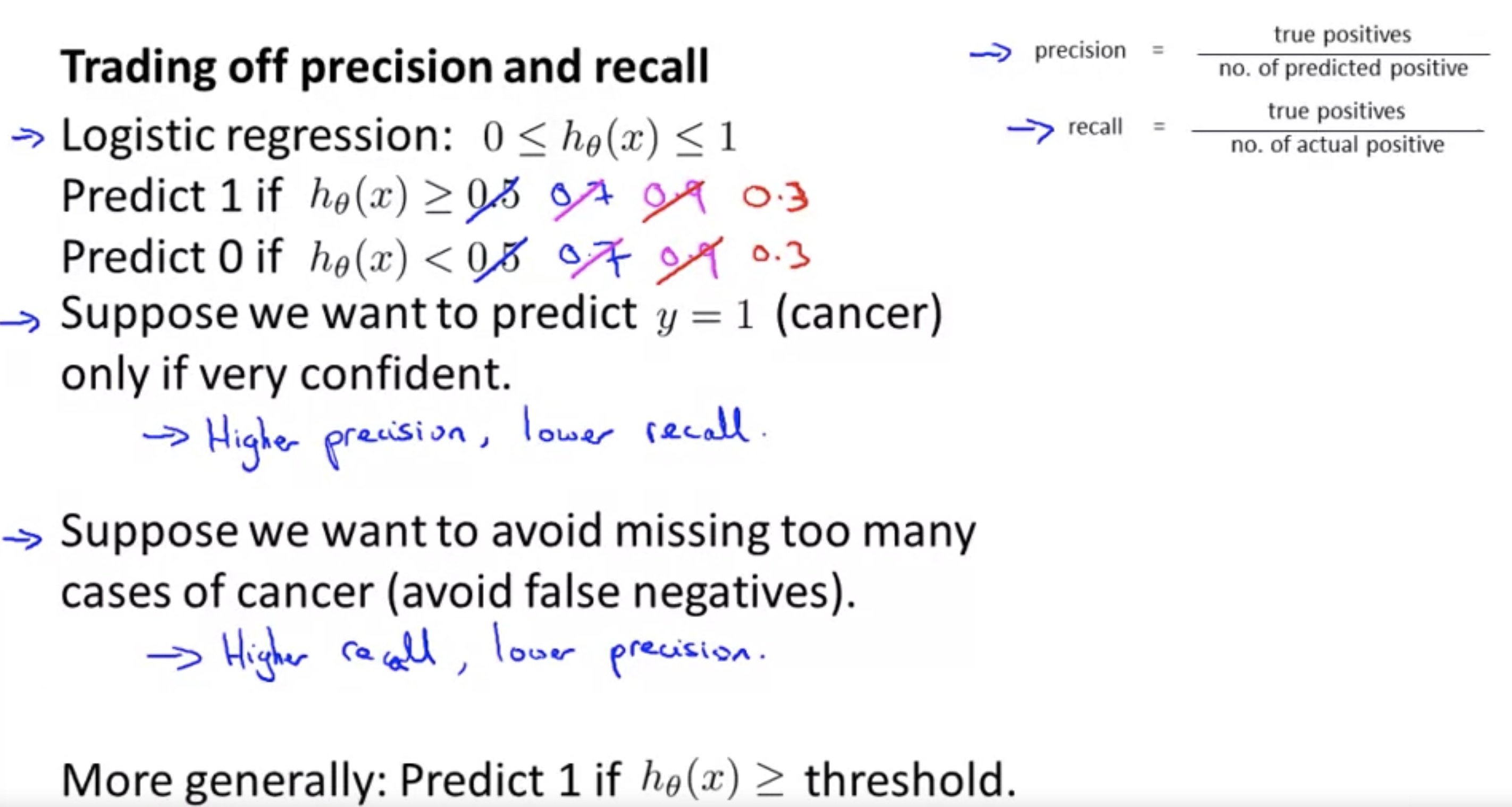
Precision:

\[\frac{\# True ~Positives}{\#~ Total~Predicted~Positives}\]

Recall:

\[\frac{\# True ~Positives}{\#~ Total~Actual~Positives}\]

Trading off precision and recall

How do we compare precision/recall numbers?

\[\begin{array}{l|cc}\hline & {\text { Precision℗ }} & {\text { Recall }(\mathrm{R})} \\ \hline \text { Algorithm } & {0.5} & {0.4} \\ {\text { Algorithm } 2} & {0.7} & {0.1} \\ {\text { Algorithm } 3} & {0.02} & {1.0}\end{array}\]

It is a bad idea to use average of these two scores. Since if we predict y=1 all the time, then recall will be 1. the average is one, which is still very high.

We use F1 score to measure overall accuracy, when both precision and recall are involved. $F_1 ~ Score=2 \frac{PR}{P+R}$

My thoughts: since we can always directly output the result $h_\Theta(x)$. The final classification is more of a problem of deciding wether to take some actins. Therefore, it would be better to calculate the gain/loss of the precision/recall. i.e.:

• the cost associated with actions on false positives
• the cost due to no precautions on false negatives.

Data for Machine Learning

Large number of features/hidden layers, and the features do have the ability to predict the result (as human expert did)–> low $J_{train}(\Theta)$; Large number of training examples –> $J_{train}(\Theta)\approx J_{test}(\Theta)$, i.e., not overfitting;

In conclusion, with large training set and many features/hidden layers, we will have good prediction.

My thoughts: can a human expert make the right prediction with the features provided?

The problem is, for many problems, the human expert rely on their computer models to predict.