Machine Learning Part 4：Support Vector Machine (SVM)

All of this series is mainly based on the Machine Learning course given by Andrew Ng, which is hosted on cousera.org.

Support Vector Machine - Linear SVM

the cost function for SVM is:

\[\min _{\theta} ~~~C \sum_{i=1}^{m}\left[y^{(i)} \operatorname{cost}_{1}\left(\theta^{T} x^{(i)}\right)+\left(1-y^{(i)}\right) \operatorname{cost}_{0}\left(\theta^{T} x^{(i)}\right)\right]+\frac{1}{2} \sum_{i=1}^{n} \theta_{j}^{2}\]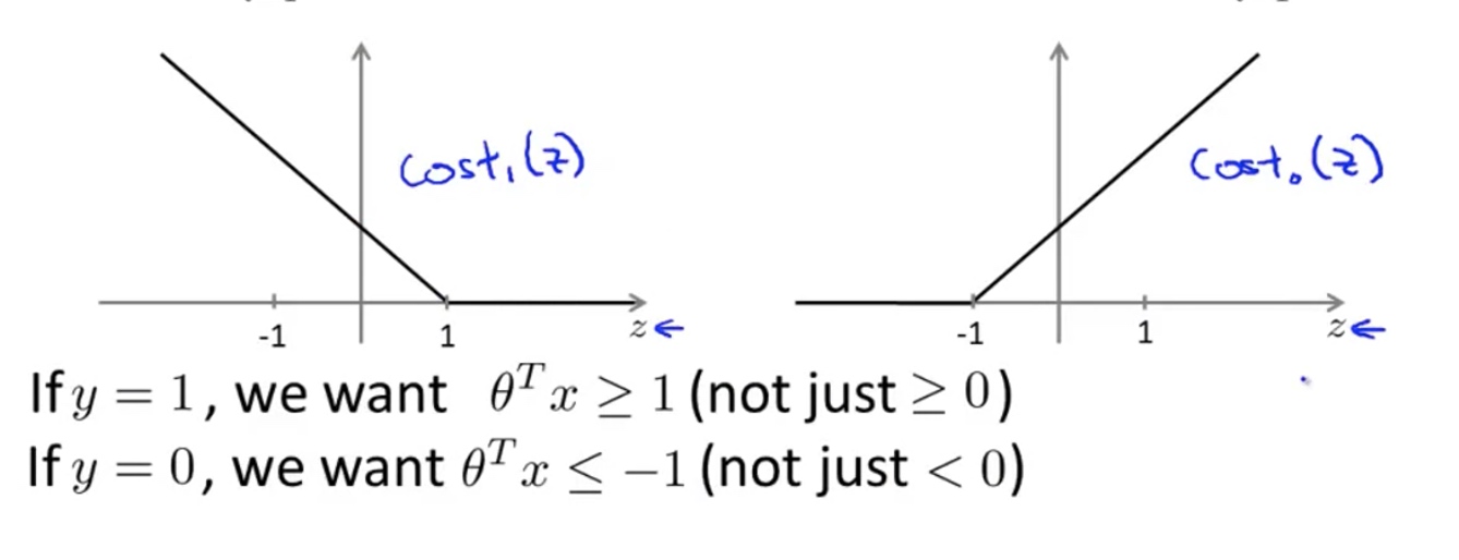

Note: C is like $\frac{1}{\lambda}$ in the logistic regression model:

\[\min _{\theta}~~ -\frac{1}{m} \sum_{i=1}^{m}\left[y^{(i)} log\left(h_\theta( x^{(i)})\right)+\left(1-y^{(i)}\right) log\left(1-h_\theta( x^{(i)})\right)\right]+\frac{\lambda}{2m} \sum_{j=1}^{n} \theta_{j}^{2}\]

SVM is also called Large Margin Classifier

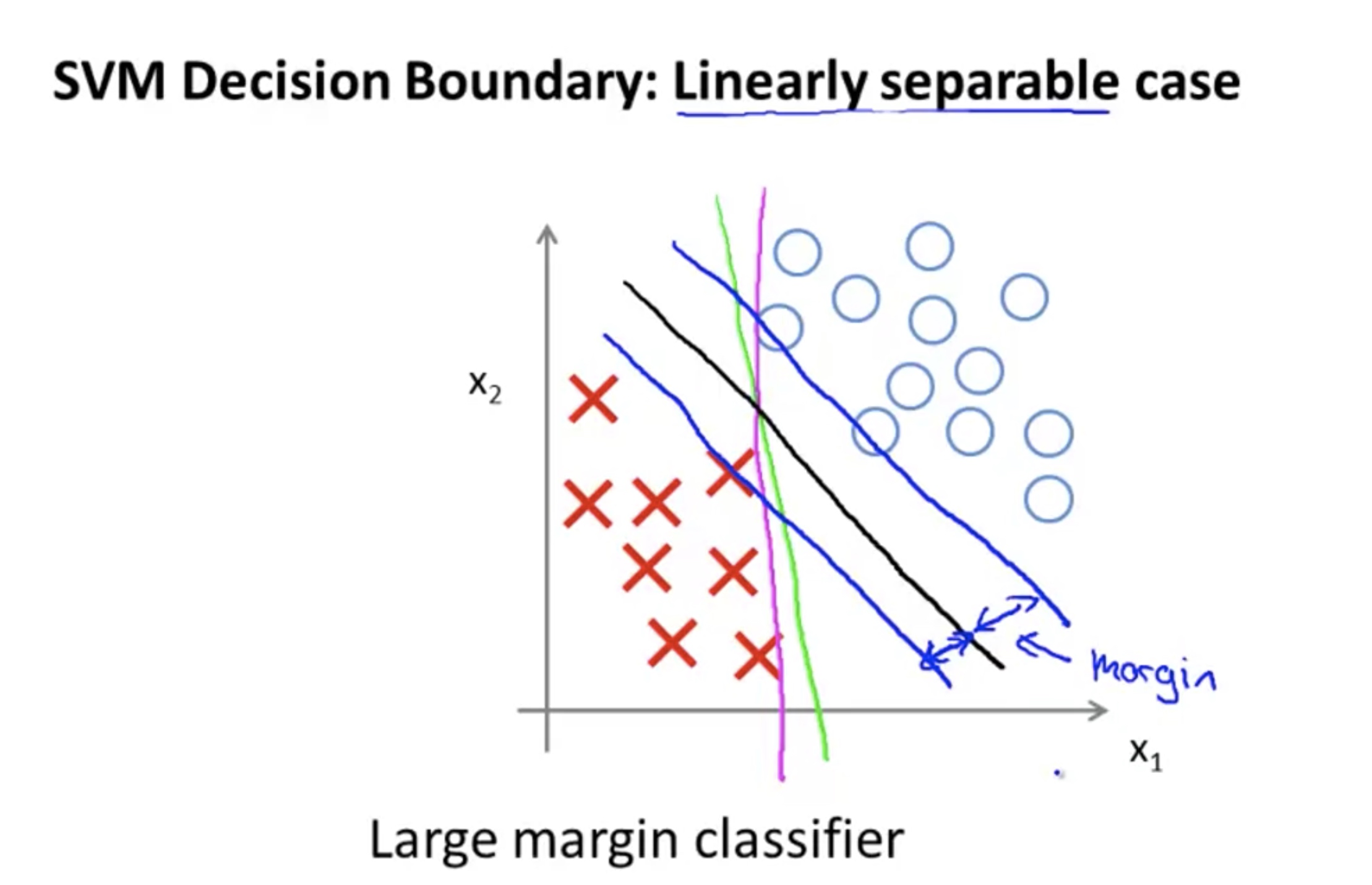
Mathematics Behind Large Margin Classification

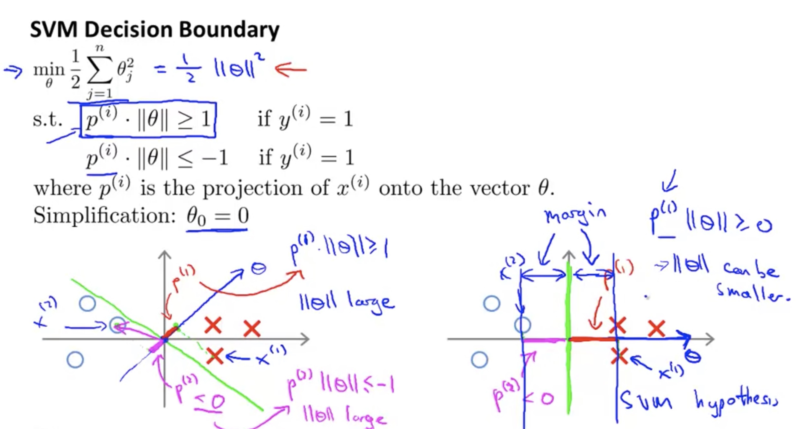
when try to find the optimum, the $\theta$ has two dimension: the angle, and the length;

since the objective is to minimize the length, the optimum tends to be that can separate the two classes with the angel to be as parallel as possible with (class1 $\to$ class2); in this case, the resulting line is the green one in the picture.

In fact, the smaller the $||\theta ||$, the bigger the margin distance $\frac{b}{||\theta ||}$.

Hard Margin

If the training data is linearly separable, we can select two parallel hyperplanes that separate the two classes of data, so that the distance between them is as large as possible.

We can put this together to get the optimization problem:

“Minimize ${\displaystyle |{\vec {w}}|}$ subject to ${\displaystyle y_{i}({\vec {w}}\cdot {\vec {x}}_{i}-b)\geq 1}$ for ${\displaystyle i=1,\ldots ,n}$” The ${\vec {w}}$ and b that solve this problem determine our classifier, ${\displaystyle {\vec {x}}\mapsto \operatorname {sgn}({\vec {w}}\cdot {\vec {x}}-b)}.$

An important consequence of this geometric description is that the max-margin hyperplane is completely determined by those ${\displaystyle{\vec {x}}{i}}$ that lie nearest to it. These ${\displaystyle{\vec {x}}{i}}$ are called support vectors.

Soft Margin

To extend SVM to cases in which the data are not linearly separable, we introduce the hinge loss function,

\[{\displaystyle \max \left(0,1-y_{i}({\vec {w}}\cdot {\vec {x}}_{i}-b)\right).}\]

This function is zero if the constraint in (1) is satisfied, in other words, if ${\vec {x}}_{i}$ lies on the correct side of the margin. For data on the wrong side of the margin, the function’s value is proportional to the distance from the margin. we then wish to minimize:

\[{\displaystyle \left[{\frac {1}{n}}\sum _{i=1}^{n}\max \left(0,1-y_{i}({\vec {w}}\cdot {\vec {x}}_{i}-b)\right)\right]+\lambda \lVert {\vec {w}}\rVert ^{2}}\]

Here y=1 or -1;

If we set y=1 or 0, we get the alternative expression:

\[\min _{\theta} ~~~C \sum_{i=1}^{m}\left[y^{(i)} \operatorname{cost}_{1}\left(\theta^{T} x^{(i)}\right)+\left(1-y^{(i)}\right) \operatorname{cost}_{0}\left(\theta^{T} x^{(i)}\right)\right]+\frac{1}{2} \sum_{i=1}^{n} \theta_{j}^{2}\]

where the parameter $\lambda$ determines the trade-off between increasing the margin size and ensuring that the ${\vec {x}}_{i}$ lie on the correct side of the margin. Thus, for sufficiently small values of $\lambda$, the second term in the loss function will become negligible, hence, it will behave similar to the hard-margin SVM, if the input data are linearly classifiable, but will still learn if a classification rule is viable or not.

Nonlinear SVM

The original maximum-margin hyperplane algorithm proposed by Vapnik in 1963 constructed a linear classifier. However, in 1992, Bernhard E. Boser, Isabelle M. Guyon and Vladimir N. Vapnik suggested a way to create nonlinear classifiers by applying the kernel trick (originally proposed by Aizerman et al.[15]) to maximum-margin hyperplanes.

The resulting algorithm is formally similar, except that every dot product is replaced by a nonlinear kernel function. This allows the algorithm to fit the maximum-margin hyperplane in a transformed feature space. The transformation may be nonlinear and the transformed space high-dimensional; although the classifier is a hyperplane in the transformed feature space, it may be nonlinear in the original input space.

It is noteworthy that working in a higher-dimensional feature space increases the generalization error(High Variance) of support-vector machines, although given enough samples the algorithm still performs well.

Some common kernels include:

Polynomial (homogeneous): ${\displaystyle k({\vec {x_{i}}},{\vec {x_{j}}})=({\vec {x_{i}}}\cdot {\vec {x_{j}}})^{d}}$

Polynomial (inhomogeneous): ${\displaystyle k({\vec {x_{i}}},{\vec {x_{j}}})=({\vec {x_{i}}}\cdot {\vec {x_{j}}}+1)^{d}}$

Gaussian radial basis function: ${\displaystyle k({\vec {x_{i}}},{\vec {x_{j}}})=\exp(-\gamma |{\vec {x_{i}}}-{\vec {x_{j}}}|^{2})}.$ Sometimes parametrized using ${\displaystyle \gamma =1/(2\sigma ^{2})}.$

Kernels

For Non-linear Decision Boundary, we can add polynomial of existing features:

Other options than polynomials? Kernel There are many forms of kernels. Here is Gaussian Kernels: For landmark $l$, define the kernel as:

\[f_l=\text{similarity}(x,l)=\exp \left(-\frac{||x-l||^2}{2\sigma^2}\right)\]

we can choose many landmarks and create the associated features. In essence, it adds another dimension of “height” to the existing feature space. So that we can separate a point from its locally adjacent domain.

With smaller $\sigma$, the height decrease more quickly, and the it’s easier to separate the landmark from nearby space.

SVM with kernels

\[\begin{array}{l}{\text { Given }\left(x^{(1)}, y^{(1)}\right),\left(x^{(2)}, y^{(2)}\right), \ldots,\left(x^{(m)}, y^{(m)}\right)} \\ {\text { choose } l^{(1)}=x^{(1)}, l^{(2)}=x^{(2)}, \ldots, l^{(m)}=x^{(m)}}\end{array}\] \[\begin{array}{l}{\text { Given example } x :} \\ {\qquad \begin{array}{l}{f_{1}=\operatorname{similarity}\left(x, l^{(1)}\right)} \\ {f_{2}=\operatorname{similarity}\left(x, l^{(2)}\right)} \\ {\ldots}\end{array}}\end{array}\]

we replace the original features $X^{(i)}\in \mathcal{R}^{n+1}$ by $f^{(i)} \in \mathcal{R}^{m+1}$, in the following ways:

$f^{(i)}_j=similarity(x^{(i)},l^{(j)}), for ~j\in[1,…,m],i\in[1,…,m]$ $f^{(i)}_0 =1$ and $f^{(0)} =1$

Definition of the SVM with Kernels

Hypothesis: Given x, compute features $f\in R^{m+1}$ Predict “y=1” if $\theta*f \geq 0$.

Training:

\[\min _{\theta} C \sum_{i=1}^{m} y^{(i)} \operatorname{cost}_{1}\left(\theta^{T} f^{(i)}\right)+\left(1-y^{(i)}\right) \operatorname{cost}_{0}\left(\theta^{T} f^{(i)}\right)+\frac{1}{2} \sum_{j=1}^{m} \theta_{j}^{2}\]

SVM Parameters

$C=\frac{1}{\lambda}$ Large C: low bias, high variance, overfitting Small C: high bias, low variance, underfitting

$\sigma^2$: Large $\sigma$: more smooth kernels, high bias, low variance Small $\sigma$: less smooth kernels, low bias, high variance

Using An SVM

• use SVM software package (e.g., liblinear, libsvm) to solve for parameters $\theta$
• need to specify the $C$ and the choice of kernel, and $\sigma$. e.g.:

\[\begin{array}{l}{\text { Gaussian kernel: }} \\ {\qquad f_{i}=\exp \left(-\frac{\left\|x-l^{(i)}\right\|^{2}}{2 \sigma^{2}}\right), \text { where } l^{(i)}=x^{(i)}}\end{array}\]

For most solvers, we need to define the kernel(similarity) function:

\[\begin{array}{l}{\text { function } \mathrm{f}=\text { kernel }(\mathrm{x} 1, \mathrm{x} 2)} \\ {\qquad f=\exp \left(-\frac{\| \times 1-\mathrm{x} 2\|^{2}}{2 \sigma^{2}}\right)} \\ {\text { return }}\end{array}\]

And we need to do feature scaling before using the Gaussian kernel $||x-l||^2=\sum_j (x_j-l_j)^2$. Without feature scaling, some of the small features will be dominated by the other bigger features.

Since the kernels replace the original $X \in R^{m\times n}$ by $f \in R^{m\times m}$, the linear kernel(No kernel) will incorporate more data if $n»m$. On the other hand, if we have a lot of training examples, $m»n$, than the f will have more information.

• n>=m: use logistic regression, or SVM without a kernel (linear kernel)
• If n is small, m is intermediate (1~50000): use SVM with Gaussian Kernel
• if n is small, m is large: create/add more features, then use logisitic regression or SVM without a kernel
• Neural network is likely to work well for most of these settings, but may be slower to train.

Multi-Class Classification

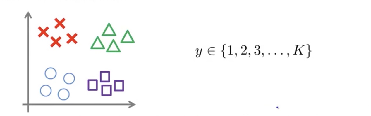
Many SVM packages already have built-in multi-class classification functionality. Otherwise, use On-vs-all method.