
All of this series is mainly based on the Machine Learning course given by Andrew Ng, which is hosted on cousera.org.
Neural Networks: Representation
Model Representation I
In neural networks, we use the same logistic function as in classification, $\frac{1}{1 + e^{-\theta^Tx}}$, yet we sometimes call it a sigmoid (logistic) activation function. In this situation, our “theta” parameters are sometimes called “weights”.
Visually, a simplistic representation looks like:
\[\left[\begin{array}{l}{x_{0}} \\ {x_{1}} \\ {x_{2}}\end{array}\right] \rightarrow[\quad] \rightarrow h_{\theta}(x)\]Our input nodes (layer 1), also known as the “input layer”, go into another node (layer 2), which finally outputs the hypothesis function, known as the “output layer”.
We can have intermediate layers of nodes between the input and output layers called the “hidden layers.”
In this example, we label these intermediate or “hidden” layer nodes $a_{0}^{2} \cdots a_{n}^{2}$ and call them “activation units.”
\[\begin{array}{l}{a_{i}^{(j)}=\text { "activation" of unit } i \text { in layer } j} \\ {\Theta^{(j)}=\text { matrix of weights controlling function mapping from layer } j \text { to layer } j+1}\end{array}\]If we had one hidden layer, it would look like:
\[\left[\begin{array}{l}{x_{0}} \\ {x_{1}} \\ {x_{2}} \\ {x_{3}}\end{array}\right] \rightarrow\left[\begin{array}{l}{a_{1}^{(2)}} \\ {a_{2}^{(2)}} \\ {a_{3}^{(2)}}\end{array}\right] \rightarrow h_{\theta}(x)\]The values for each of the “activation” nodes is obtained as follows:
\[\begin{array}{r}{a_{1}^{(2)}=g\left(\Theta_{10}^{(1)} x_{0}+\Theta_{11}^{(1)} x_{1}+\Theta_{12}^{(1)} x_{2}+\Theta_{13}^{(1)} x_{3}\right)} \\ {a_{2}^{(2)}=g\left(\Theta_{20}^{(1)} x_{0}+\Theta_{21}^{(1)} x_{1}+\Theta_{22}^{(1)} x_{2}+\Theta_{23}^{(1)} x_{3}\right)} \\ {a_{3}^{(2)}=g\left(\Theta_{30}^{(1)} x_{0}+\Theta_{31}^{(1)} x_{1}+\Theta_{32}^{(1)} x_{2}+\Theta_{33}^{(1)} x_{3}\right)} \\ {h_{\Theta}(x)=a_{1}^{(3)}=g\left(\Theta_{10}^{(2)} a_{0}^{(2)}+\Theta_{11}^{(2)} a_{1}^{(2)}+\Theta_{12}^{(2)} a_{2}^{(2)}+\Theta_{13}^{(2)} a_{3}^{(2)}\right)}\end{array}\]This is saying that we compute our activation nodes by using a 3×4 matrix of parameters. We apply each row of the parameters to our inputs to obtain the value for one activation node. Our hypothesis output is the logistic function applied to the sum of the values of our activation nodes, which have been multiplied by yet another parameter matrix $\mathbf{\Theta}^{(2)}$ containing the weights for our second layer of nodes.
Each layer gets its own matrix of weights, $\Theta^{(j)}$.
The dimensions of these matrices of weights is determined as follows:
If network has sj units in layer j and $s_{j+1}$ units in layer j+1, then $\Theta^{(j)}$ will be of dimension $s_{j+1}*(s_{j}+1)$.
The +1 comes from the addition in $\Theta^{(j)}$ of the “bias nodes,” $x_0$.
Model Representation II
In this section we’ll do a vectorized implementation of the above functions. We’re going to define a new variable $z_k^{(j)}$ that encompasses the parameters inside our g function. In our previous example if we replaced by the variable z for all the parameters we would get:
$\begin{aligned} a_{1}^{(2)} &=g\left(z_{1}^{(2)}\right) \ a_{2}^{(2)} &=g\left(z_{2}^{(2)}\right) \ a_{3}^{(2)} &=g\left(z_{3}^{(2)}\right) \end{aligned}$
In other words, for layer j=2 and node k, the variable z will be:
$z_{k}^{(2)}=\Theta_{k, 0}^{(1)} x_{0}+\Theta_{k, 1}^{(1)} x_{1}+\cdots+\Theta_{k, n}^{(1)} x_{n}$
The vector representation of x and $z^{j}$ is:
$x=\left[\begin{array}{l}{x_{0}} \ {x_{1}} \ {\cdots} \ {x_{n}}\end{array}\right] z^{(j)}=\left[\begin{array}{c}{z_{1}^{(j)}} \ {z_{2}^{(j)}} \ {\cdots} \ {z_{n}^{(j)}}\end{array}\right]$
Setting $x = a^{(1)}$, we can rewrite the equation as:
$z^{(j)}=\Theta^{(j-1)} a^{(j-1)}$
Now we can get a vector of our activation nodes for layer j as follows:
$a^{(j)}=g(z^{(j)})=g(\Theta^{(j-1)} a^{(j-1)})$
We can then add a bias unit (equal to 1) to layer j after we have computed $a^{(j)}$. This will be element $a_0^{(j)}$ and will be equal to 1. To compute our final hypothesis, let’s first compute another z vector:
$z^{(j+1)}=\Theta^{(j)} a^{(j)}$
This last theta matrix $\Theta^{(j)}$ will have only one row which is multiplied by one column $a^{(j)}$ so that our result is a single number. We then get our final result with:
$h_{\Theta}(x)=a^{(j+1)}=g(z^{(j+1)})$
Notice that in this last step, between layer j and layer j+1, we are doing exactly the same thing as we did in logistic regression. Adding all these intermediate layers in neural networks allows us to more elegantly produce interesting and more complex non-linear hypotheses.
Examples and Intuitions
The graph of our functions will look like:
$\left[\begin{array}{l}{x_{0}} \ {x_{1}} \ {x_{2}}\end{array}\right] \rightarrow\left[g\left(z^{(2)}\right)\right] \rightarrow h_{\Theta}(x)$
Remember that $ x_0$ is our bias variable and is always 1.
Let’s set our first theta matrix as:
And
Θ(1)=[−30, 20, 20]
This will cause the output of our hypothesis to only be positive if both $x_1$ and $x_2$ are 1. In other words:
\[\begin{array}{l}{h_{\Theta}(x)=g\left(-30+20 x_{1}+20 x_{2}\right)} \\ {x_{1}=0 \text { and } x_{2}=0 \text { then } g(-30) \approx 0} \\ {x_{1}=0 \text { and } x_{2}=1 \text { then } g(-10) \approx 0} \\ {x_{1}=1 \text { and } x_{2}=0 \text { then } g(-10) \approx 0} \\ {x_{1}=1 \text { and } x_{2}=1 \text { then } g(10) \approx 1}\end{array}\]Or
Θ(1)=[−10, 20, 20]
Not X
Θ(1)=[10, -20]
Not $X_1$ and Not $X_2$
Θ(1)=[10, -20, -20]
Multiclass Classification
To classify data into multiple classes, we let our hypothesis function return a vector of values. Say we wanted to classify our data into one of four categories. We will use the following example to see how this classification is done. This algorithm takes as input an image and classifies it accordingly:
We can define our set of resulting classes as y:
\[y^{(i)}=\left[\begin{array}{l}{1} \\ {0} \\ {0} \\ {0}\end{array}\right],\left[\begin{array}{l}{0} \\ {1} \\ {0} \\ {0}\end{array}\right],\left[\begin{array}{l}{0} \\ {0} \\ {1} \\ {0}\end{array}\right],\left[\begin{array}{l}{0} \\ {0} \\ {0} \\ {1}\end{array}\right]\]Each $y^{(i)}$ represents a different image corresponding to either a car, pedestrian, truck, or motorcycle. The inner layers, each provide us with some new information which leads to our final hypothesis function. The setup looks like:
\[\left[\begin{array}{l}{x_{0}} \\ {x_{1}} \\ {x_{2}} \\ {\cdots} \\ {x_{n}}\end{array}\right] \rightarrow\left[\begin{array}{c}{a_{0}^{(2)}} \\ {a_{1}^{(2)}} \\ {a_{2}^{(2)}} \\ {\cdots}\end{array}\right] \rightarrow\left[\begin{array}{c}{a_{0}^{(3)}} \\ {a_{1}^{(3)}} \\ {a_{2}^{(3)}} \\ {\cdots}\end{array}\right] \rightarrow \cdots \rightarrow\left[\begin{array}{l}{h_{\Theta}(x)_{1}} \\ {h_{\Theta}(x)_{2}} \\ {h_{\Theta}(x)_{3}} \\ {h_{\Theta}(x)_{4}}\end{array}\right]\]Our resulting hypothesis for one set of inputs may look like:
$h_\Theta(x)=\left[\begin{array}{l}{0} \ {0} \ {1} \ {0}\end{array}\right]$
In which case our resulting class is the third one down, or $h_\Theta(x)_3=1$, which represents the motorcycle.
Neural Networks: Learning
Cost Function
Let’s first define a few variables that we will need to use:
- L = total number of layers in the network
- $s_l$ = number of units (not counting bias unit) in layer l
- K = number of output units/classes
Recall that in neural networks, we may have many output nodes. We denote $h_\Theta(x)_k$ as being a hypothesis that results in the $k^{th}$ output. Our cost function for neural networks is going to be a generalization of the one we used for logistic regression. Recall that the cost function for regularized logistic regression was:
$J(\theta)=-\frac{1}{m} \sum_{i=1}^{m}\left[y^{(i)} \log \left(h_{\theta}\left(x^{(i)}\right)\right)+\left(1-y^{(i)}\right) \log \left(1-h_{\theta}\left(x^{(i)}\right)\right)\right]+\frac{\lambda}{2 m} \sum_{j=1}^{n} \theta_{j}^{2}$
For neural networks, it is going to be slightly more complicated:
\[J(\Theta)=-\frac{1}{m} \sum_{i=1}^{m} \sum_{k=1}^{K}\left[y_{k}^{(i)} \log \left(\left(h_{\Theta}\left(x^{(i)}\right)\right)_{k}\right)+\left(1-y_{k}^{(i)}\right) \log \left(1-\left(h_{\Theta}\left(x^{(i)}\right)\right)_{k}\right)\right]+\frac{\lambda}{2 m} \sum_{l=1}^{L-1} \sum_{i=1}^{s_{l}} \sum_{j=1}^{s_{l+1}}\left(\Theta_{j, i}^{(l)}\right)^{2}\]Note:
-
For each layer, we do not regularize the $\Theta_{j,0}$, just like we do not regularize the $\theta_0$ in the logistic regression.
-
Therefore, even though $\Theta^{(l)}$ is a $s_{j+1}*(s_{j}+1)$ matrix, we do not regularize on the first column $\Theta(:,1)$.
Backpropagation Algorithm
“Backpropagation” is neural-network terminology for minimizing our cost function, just like what we were doing with gradient descent in logistic and linear regression. Our goal is to compute:
$\min_\Theta J(\Theta)$
That is, we want to minimize our cost function J using an optimal set of parameters in theta. In this section we’ll look at the equations we use to compute the partial derivative of J(Θ):
\[\begin{equation} \frac{\partial}{\partial \Theta_{i, j}^{(l)}} J(\Theta) \end{equation}\]To do so, we use the following algorithm:
Back propagation Algorithm:
Given training set
\[\begin{equation} \left\{\left(x^{(1)}, y^{(1)}\right) \cdots\left(x^{(m)}, y^{(m)}\right)\right\} \end{equation}\]- Set $\Delta^{(l)}_{i,j}=0$ for all (l,i,j), (hence you end up having a matrix full of zeros)
For training example t =1 to m:
- Set $a^{(1)}:=x^{(t)}$
- Perform forward propagation to compute $a^{(l)}$ for l=2,3,…,L
- Using $y^{(t)}$, compute $\delta^{(L)} = a^{(L)} - y^{(t)}$
Where L is our total number of layers and $a^{(L)}$ is the vector of outputs of the activation units for the last layer. So our “error values” for the last layer are simply the differences of our actual results in the last layer and the correct outputs in y. To get the delta values of the layers before the last layer, we can use an equation that steps us back from right to left:
- Compute $\delta^{(L-1)}, \delta^{(L-2)},\dots,\delta^{(2)}$ using $\begin{equation} \delta^{(l)}=\left(\left(\Theta^{(l)}\right)^{T} \delta^{(l+1)}\right).*g’(z^{(l)}) \end{equation}$
Since $g’(z^{(l)})= a^{(l)} \cdot *\left(1-a^{(l)}\right)$
$\begin{equation} \delta^{(l)}=\left(\left(\Theta^{(l)}\right)^{T} \delta^{(l+1)}\right)\cdot * a^{(l)} \cdot *\left(1-a^{(l)}\right) \end{equation}$
-
$\begin{equation} \Delta_{i, j}^{(l)} :=\Delta_{i, j}^{(l)}+ \delta_{i}^{(l+1)}a_{j}^{(l)} \end{equation}$ or with vectorization, $\Delta^{(l)} := \Delta^{(l)} + \delta^{(l+1)}(a^{(l)})^T$
- Note, we need to remove the $\delta_0^{(l)}$ for $l<L$ for the calculation of $\Delta^{(l)}$;
- This is because the $\Delta_{i, j}^{(l)}$ should have dimension of $s_{l+1}\times s_{l}+1$
- But for $l+1<L$, $\delta^{(l+1)}$ has dimension of $s_{l+1}+1$. Therefore, we should delete this term.
Hence we update our new $\Delta$ matrix:
\[\begin{array}{l}{ D_{i, j}^{(l)} :=\frac{1}{m}\sum_{all~examples} \left(\Delta_{i, j}^{(l)}+\lambda \Theta_{i, j}^{(l)}\right), \text { if } j \neq 0} \\ { D_{i, j}^{(l)} :=\frac{1}{m} \sum_{all~examples} \Delta_{i, j}^{(l)} \text { , lf } j=0}\end{array}\]The capital-delta matrix D is used as an “accumulator” to add up our values as we go along and eventually compute our partial derivative. Thus we get
$\begin{equation} \frac{\partial}{\partial \Theta_{i, j}^{(l)}} J(\Theta) \end{equation}= D_{i, j}^{(l)}$.
Mathematical Intuition:

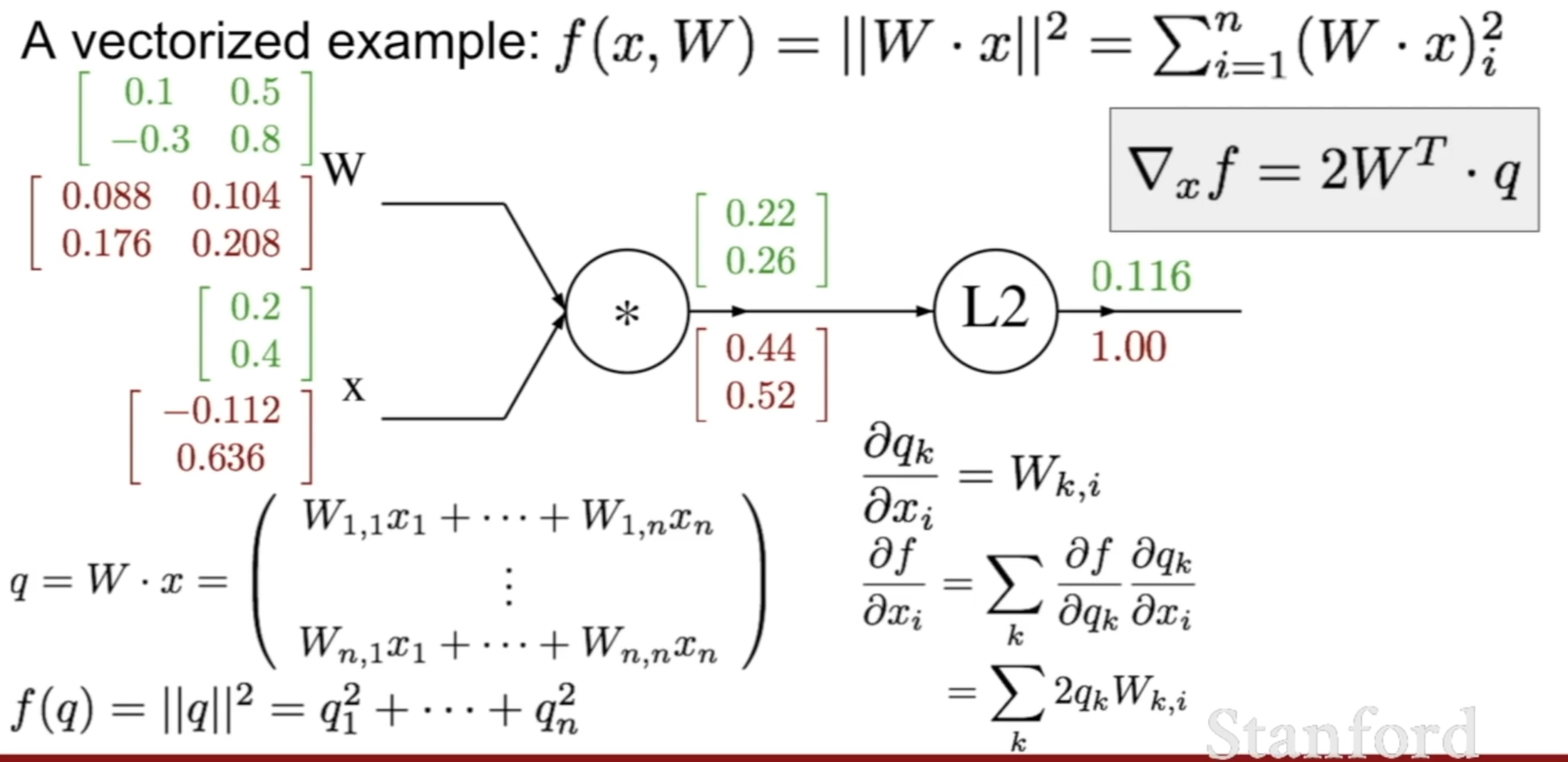
For L2 norm or linear regression problem: $W\in R^{m\times n}, x \in R^n , y\in R^n$ $f(x, W)=|W \cdot x|^{2}=\sum_{i=1}^{n}(W \cdot x)_{i}^{2}$, then we have:
\[\nabla_{W} f=2 q \cdot x^{T} \\\nabla_{x} f=2 W^{T} \cdot q\]Note: the gradient w.r.t. any matrix/vector has the same shape with the matrix/vector.
For Logistic regression Problem: $W\in R^{m\times n}, x \in R^n , y\in R^n$ $f(x, W)=-[(1-y) \cdot log(1-Sigmoid(W\cdot x))+y\cdot log(Sigmoid(W\cdot x)) ]$, then we have:
\[\nabla_{W} f= q \cdot x^{T} \\\nabla_{x} f= W^{T} \cdot q\]$W\in R^{1 \times n}, x \in R^{n \times 1} , y\in R^1$ $f(x, W)=W\cdot x$, then we have:
\[\nabla_{W} f= X^T \\\nabla_{x} f= W^{T}\]$J(\Theta)=J(\Theta^{L-1}; a^{L-1})$ ;Where $a^{L-1}=g(\Theta^{L-2}*a^{L-2})$
$\frac{\partial J}{\partial \Theta^{L-1}}$ is just the like $\nabla_{W} f= q \cdot x^{T}$:
\[\frac{\partial J}{\partial \Theta^{L-1}}=\delta^L*\left( a^{L-1}\right)^{T}\]Similar to the fact $\nabla_{x} f= W^{T} \cdot q$
\[\frac{\partial J}{\partial a^{l-1}}=(\Theta^{L-1})^T(g(X\theta)-y)=(\Theta^{(L-1)})^T *\delta^{L}\\\]And for previous $\Theta^{L-2}$, since $a^{L-1}=g(\Theta^{L-2}*a^{L-1})$ is a function of $\Theta^{L-2}$, we can use the chain rule to derive the $\frac{\partial J}{\partial \Theta^{L-2}}$ as:
\[\begin{array}{lcl} \frac{\partial J}{\partial \Theta^{L-2}}&=&\frac{\partial J}{\partial a^{L-1}}*\frac{\partial a^{L-1}}{\partial \Theta^{L-2}} \\&=&(\Theta^{L-1})^T*\delta^L*g'(z^{L-1})*(a^{L-2})^T\\ &=&\delta^{L-1}*(a^{l-2})^T \end{array}\]In other words:
\[\frac{\partial J}{\partial \Theta^l}=\delta^{(l+1)}*(a^{(l)})^T \\ \delta^{(l)}=\left(\left(\Theta^{(l)}\right)^{T} \delta^{(l+1)}\right)\cdot * a^{(l)} \cdot *\left(1-a^{(l)}\right)\]Backpropagation Intuition
In the image above, to calculate $\delta_2^{(2)}$, we multiply the weights $\Theta^{(2)}_{12}$ and
\[\Theta^{(2)}_{22}\]by their respective $\delta$ values found to the right of each edge. So we get $\delta_{2}^{(2)}=\Theta_{12}^{(2)} \star \delta_{1}^{(3)}+\Theta_{22}^{(2)} \star \delta_{2}^{(3)}$. To calculate every single possible $\delta_j^{(l)}$, we could start from the right of our diagram. We can think of our edges as our $\Theta_{ij}$. Going from right to left, to calculate the value of $\delta_j^{(l)}$, you can just take the over all sum of each weight times the $\delta$ it is coming from. Hence, another example would be $\delta_2^{(3)}=\Theta^{(3)}_{12}\delta_1^{(4)}$
$Z=\Theta*X$
Since backwards, the true $\theta$, i.e. previous $\theta$, lies in $X$, the derivative will be like $(\Theta^{(l)})^T*\delta^{(l+1)}$
Backpropagation in Practice
With neural networks, we are working with sets of matrices:
\[\begin{array}{l}{\Theta^{(1)}, \Theta^{(2)}, \Theta^{(3)}, \ldots} \\ {D^{(1)}, D^{(2)}, D^{(3)}, \ldots}\end{array}\]In order to use optimizing functions such as “fminunc()”, we will want to “unroll” all the elements and put them into one long vector:
1
2
thetaVector = [ Theta1(:); Theta2(:); Theta3(:); ]
deltaVector = [ D1(:); D2(:); D3(:) ]
If the dimensions of Theta1 is 10x11, Theta2 is 10x11 and Theta3 is 1x11, then we can get back our original matrices from the “unrolled” versions as follows:
1
2
3
Theta1 = reshape(thetaVector(1:110),10,11)
Theta2 = reshape(thetaVector(111:220),10,11)
Theta3 = reshape(thetaVector(221:231),1,11)
To summarize:
- Use to vector form for the optimization algorithms
- Use the matrix form to utilize the vectorization implementation.
Gradient Checking
Gradient checking will assure that our backpropagation works as intended. We can approximate the derivative of our cost function with:
\[\frac{\partial}{\partial \Theta} J(\Theta) \approx \frac{J(\Theta+\epsilon)-J(\Theta-\epsilon)}{2 \epsilon}\]A small value for ϵ (epsilon) such as ϵ=$10^{−4}$, guarantees that the math works out properly. If the value for ϵ is too small, we can end up with numerical problems.
Hence, we are only adding or subtracting epsilon to the Θj matrix. In octave we can do it as follows:
1
2
3
4
5
6
7
8
epsilon = 1e-4;
for i = 1:n,
  thetaPlus = theta;
  thetaPlus(i) += epsilon;
  thetaMinus = theta;
  thetaMinus(i) -= epsilon;
  gradApprox(i) = (J(thetaPlus) - J(thetaMinus))/(2*epsilon)
end;
We previously saw how to calculate the deltaVector. So once we compute our gradApprox vector, we can check that gradApprox ≈ deltaVector.
Once you have verified once that your backpropagation algorithm is correct, you don’t need to compute gradApprox again. The code to compute gradApprox can be very slow.
Random Initialization
Initializing all theta weights to zero does not work with neural networks. When we backpropagate, all nodes will update to the same value repeatedly. Instead we can randomly initialize our weights for our Θ matrices using the following method:
Hence, we initialize each $\Theta^{(l)}_{ij}$ to a random value between[−ϵ,ϵ]. Using the above formula guarantees that we get the desired bound. The same procedure applies to all the Θ’s. Below is some working code you could use to experiment.
1
2
3
4
5
If the dimensions of Theta1 is 10x11, Theta2 is 10x11 and Theta3 is 1x11.

Theta1 = rand(10,11) * (2 * INIT_EPSILON) - INIT_EPSILON;
Theta2 = rand(10,11) * (2 * INIT_EPSILON) - INIT_EPSILON;
Theta3 = rand(1,11) * (2 * INIT_EPSILON) - INIT_EPSILON;
rand(x,y) is just a function in octave that will initialize a matrix of random real numbers between 0 and 1.
(Note: the epsilon used above is unrelated to the epsilon from Gradient Checking)
Putting it Together
First, pick a network architecture; choose the layout of your neural network, including how many hidden units in each layer and how many layers in total you want to have.
- Number of input units = dimension of features $x^{(i)}$
- Number of output units = number of classes
- Number of hidden units per layer = usually more the better (must balance with cost of computation as it increases with more hidden units)
- Defaults: 1 hidden layer. If you have more than 1 hidden layer, then it is recommended that you have the same number of units in every hidden layer.
Training a Neural Network
- Randomly initialize the weights
- Implement forward propagation to get $h_\Theta(x^{(i)})$ for any $x^{(i)}$
- Implement the cost function
- Implement backpropagation to compute partial derivatives
- Use gradient checking to confirm that your backpropagation works. Then disable gradient checking.
- Use gradient descent or a built-in optimization function to minimize the cost function with the weights in theta.
When we perform forward and back propagation, we loop on every training example:
1
2
3
for i = 1:m,
   Perform forward propagation and backpropagation using example (x(i),y(i))
   (Get activations a(l) and delta terms d(l) for l = 2,...,L
Codes
1
2
3
4
5
6
7
8
9
10
11
12
13
14
15
16
17
18
19
20
21
22
23
24
25
26
27
28
29
30
31
32
33
34
35
36
37
38
39
40
41
42
43
44
45
46
47
48
49
50
51
52
53
54
55
56
57
58
59
60
61
62
63
64
65
66
67
68
69
70
71
72
73
74
75
76
77
78
79
80
81
82
83
84
85
86
87
88
89
90
91
92
93
94
95
96
97
98
99
100
101
102
103
function [J grad] = nnCostFunction(nn_params, ...
                                   input_layer_size, ...
                                   hidden_layer_size, ...
                                   num_labels, ...
                                   X, y, lambda)
%NNCOSTFUNCTION Implements the neural network cost function for a two layer
%neural network which performs classification
%   [J grad] = NNCOSTFUNCTON(nn_params, hidden_layer_size, num_labels, ...
%   X, y, lambda) computes the cost and gradient of the neural network. The
%   parameters for the neural network are "unrolled" into the vector
%   nn_params and need to be converted back into the weight matrices.
%
%   The returned parameter grad should be a "unrolled" vector of the
%   partial derivatives of the neural network.
%

% Reshape nn_params back into the parameters Theta1 and Theta2, the weight matrices
% for our 2 layer neural network
Theta1 = reshape(nn_params(1:hidden_layer_size * (input_layer_size + 1)), ...
                 hidden_layer_size, (input_layer_size + 1));

Theta2 = reshape(nn_params((1 + (hidden_layer_size * (input_layer_size + 1))):end), ...
                 num_labels, (hidden_layer_size + 1));

% Setup some useful variables
m = size(X, 1);

% You need to return the following variables correctly
J = 0;
Theta1_grad = zeros(size(Theta1));
Theta2_grad = zeros(size(Theta2));

% ====================== YOUR CODE HERE ======================
% Instructions: You should complete the code by working through the
%               following parts.
%
% Part 1: Feedforward the neural network and return the cost in the
%         variable J. After implementing Part 1, you can verify that your
%         cost function computation is correct by verifying the cost
%         computed in ex4.m
%
% Part 2: Implement the backpropagation algorithm to compute the gradients
%         Theta1_grad and Theta2_grad. You should return the partial derivatives of
%         the cost function with respect to Theta1 and Theta2 in Theta1_grad and
%         Theta2_grad, respectively. After implementing Part 2, you can check
%         that your implementation is correct by running checkNNGradients
%
%         Note: The vector y passed into the function is a vector of labels
%               containing values from 1..K. You need to map this vector into a
%               binary vector of 1's and 0's to be used with the neural network
%               cost function.
%
%         Hint: We recommend implementing backpropagation using a for-loop
%               over the training examples if you are implementing it for the
%               first time.
%
% Part 3: Implement regularization with the cost function and gradients.
%
%         Hint: You can implement this around the code for
%               backpropagation. That is, you can compute the gradients for
%               the regularization separately and then add them to Theta1_grad
%               and Theta2_grad from Part 2.
%

for iter=1:m
    a1=[1;X(iter,:)'];
    yy=zeros(1,num_labels);
    yy(y(iter))=1;
    z2=Theta1*a1;
    a2=[1;sigmoid(z2)];
    z3=Theta2*a2;
    a3=sigmoid(z3);
    J=J-1/m*(yy*log(a3)+(1-yy)*log(1-a3));

    delta3=a3-yy';
    %fprintf('size of Theta2 is...[%d,%d] \n',size(Theta2))
    %fprintf('size of delta3 is...[%d,%d] \n',size(delta3))
    %fprintf('size of z2 is...[%d,%d] \n',size(z2))

    delta2= Theta2'*delta3.*[1;sigmoidGradient(z2)];
    % unless for delta Last one; other delta must delete first term;
    delta2=delta2(2:end);
    Theta2_grad = Theta2_grad + 1/m*delta3*a2';
    Theta1_grad = Theta1_grad + 1/m*delta2*a1';

end


J=J+0.5*lambda/m*(sum(nn_params.^2)-sum(Theta1(:,1).^2)-sum(Theta2(:,1).^2));

theta11=Theta1;
theta11(:,1)=0;
theta22=Theta2;
theta22(:,1)=0;

Theta2_grad = Theta2_grad + lambda/m*theta22;
Theta1_grad = Theta1_grad + lambda/m*theta11;

grad = [Theta1_grad(:) ; Theta2_grad(:)];


end
Comments