
All of this series is mainly based on the Machine Learning course given by Andrew Ng, which is hosted on cousera.org.
Unsupervised Learning – Clustering
K-means Algorithms
\[\begin{array}{l}{\text { K-means algorithm }} \\ {\text { Input: }} \\ {\qquad \begin{array}{l}{-\quad K( \text { number of clusters) } } \\ {-\quad \text { Training set }\left\{x^{(1)}, x^{(2)}, \ldots, x^{(m)}\right\}} \\ {x^{(i)} \in \mathbb{R}^{n}\left(\text { drop } x_{0}=1 \text { convention }\right)}\end{array}}\end{array}\]Algorithm:
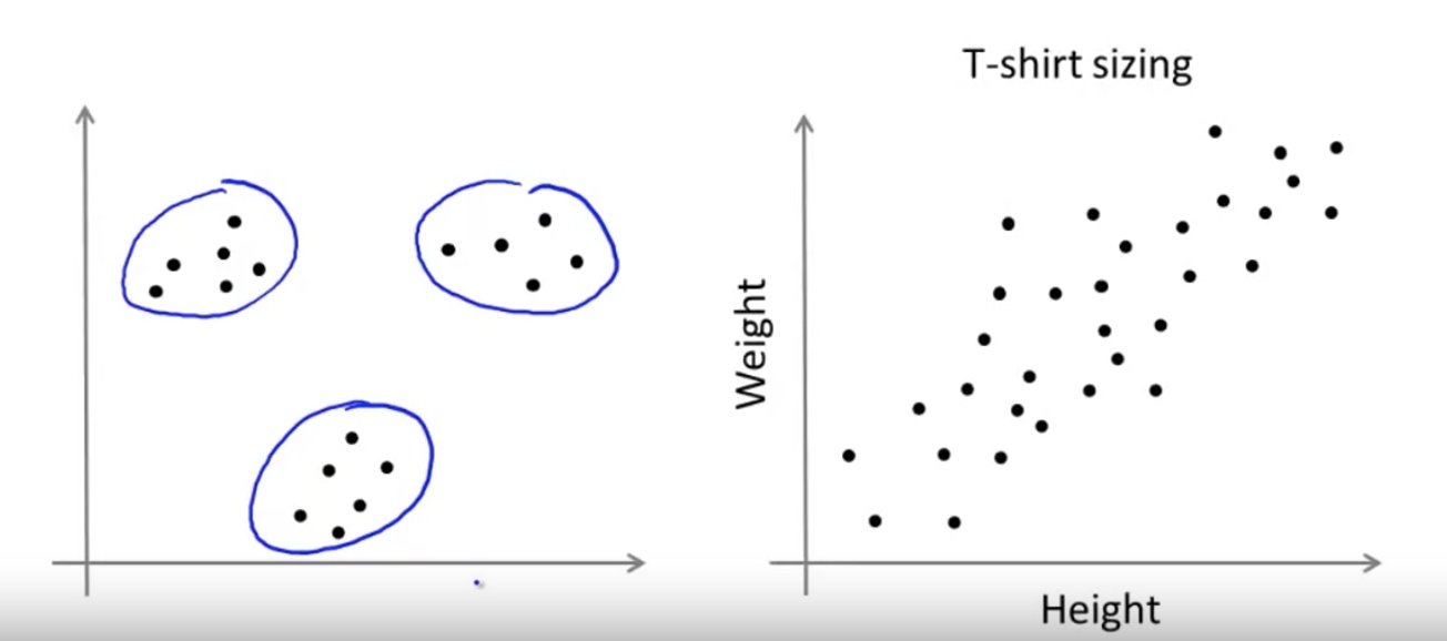
\[\begin{array}{l}{\text { K-means algorithm }} \\ {\text { Randomly initialize } K \text { cluster centroids } \mu_{1}, \mu_{2}, \ldots, \mu_{K} \in \mathbb{R}^{n}} \\ {\text { Repeat }\{} \\ {\qquad \begin{aligned}\left.c^{(i)} :=\text { index ( from } 1 \text { to } K\right) \text { of cluster centroid } \text { closest to } x^{(i)} \\ \mu_{k} :=\text { average (mean) of points assigned to cluster } k \end{aligned}} \\ {}\end{array}\]K-means for Non-separated clusters
Optimization Objective for K-means
\[\begin{array}{l}{J\left(c^{(1)}, \ldots, c^{(m)}, \mu_{1}, \ldots, \mu_{K}\right)=\frac{1}{m} \sum_{i=1}^{m}\left\|x^{(i)}-\mu_{c^{(i)}}\right\|^{2}} \\ {\min _{c^{(1)}, \ldots, c^{(m)}} J\left(c^{(1)}, \ldots, c^{(m)}, \mu_{1}, \ldots, \mu_{K}\right)} \\ {\mu_{1}, \ldots, \mu_{K}}\end{array}\]where \(\begin{aligned} c^{(i)} &=\text { index of cluster }(1,2, \ldots, K) \text { to which example } x^{(i)} \text { is currently } \\ & \text { assigned } \\ \mu_{k} &=\text { cluster centroid } k\left(\mu_{k} \in \mathbb{R}^{n}\right) \end{aligned}\)
\[\begin{aligned} \mu_{c^{(i)}} &=\text { cluster centroid of cluster to which example } x^{(i)} \text { has been } \\ & \text { assigned } \end{aligned}\]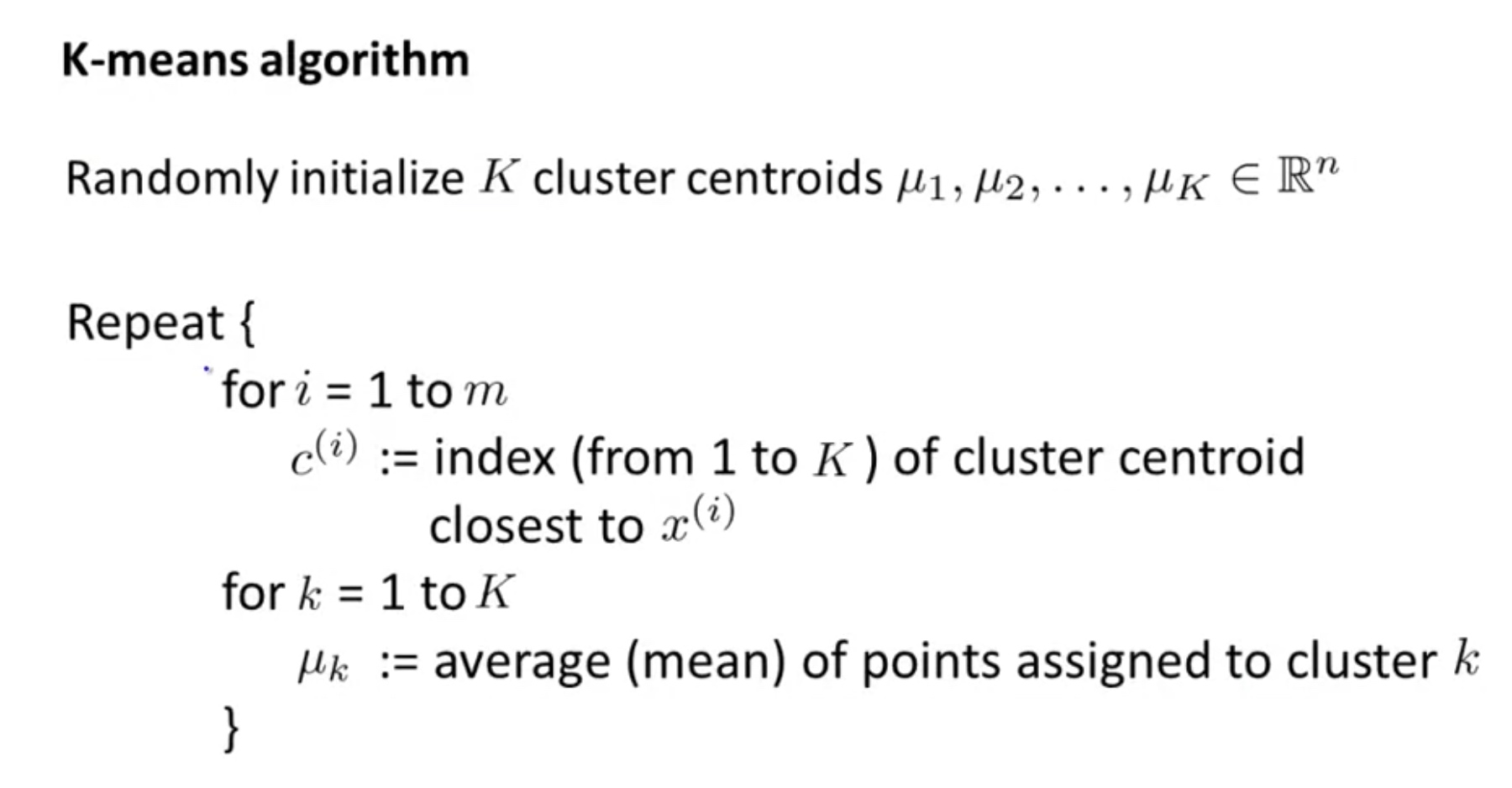
It is equivalent to repeatedly solving the optimization problem for $C^{(i)} ~for ~i=1,…,m$ first, then for $\mu_k ~for ~k=1,…,K$
Initial Guesses - Random Initialization
Bad starting point can lead to local optimum:

Solution: more trials with different starting point. Then pick the lowers cost function.
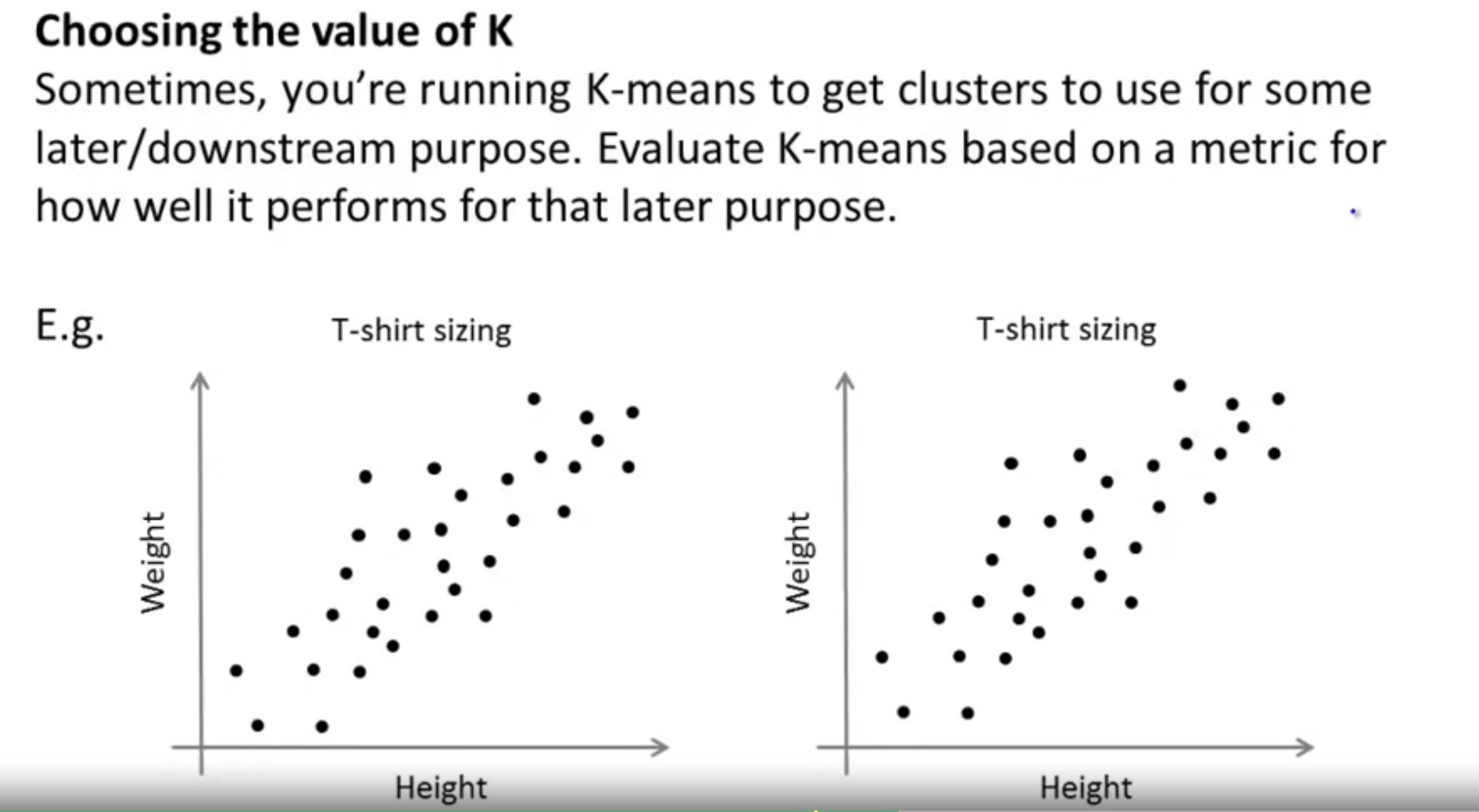
Choose the number of clusters
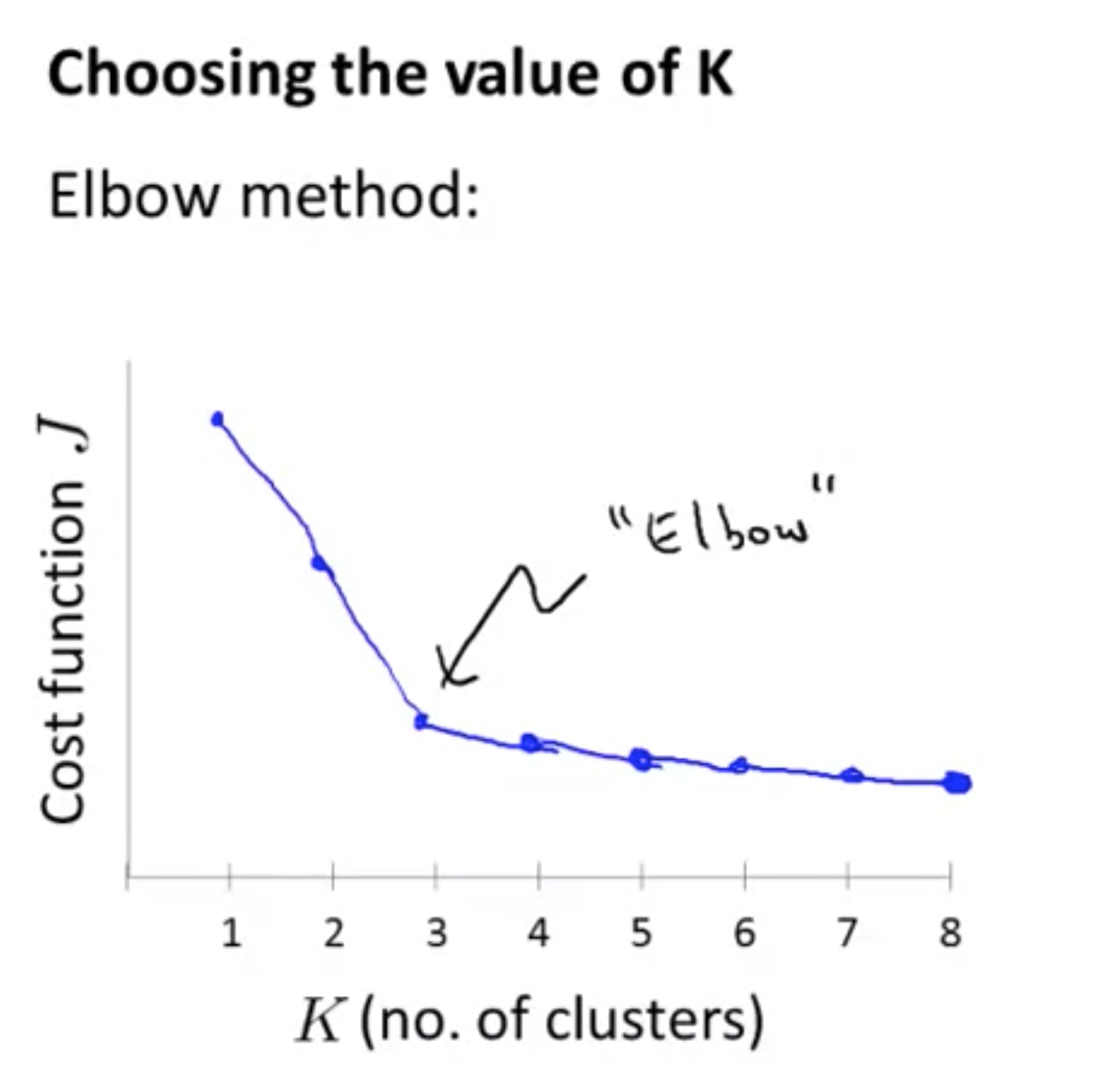
Evaluate it based on the later/downstream purposes.
Dimensionality Reduction
Motivation
- Data
- Data Visualization

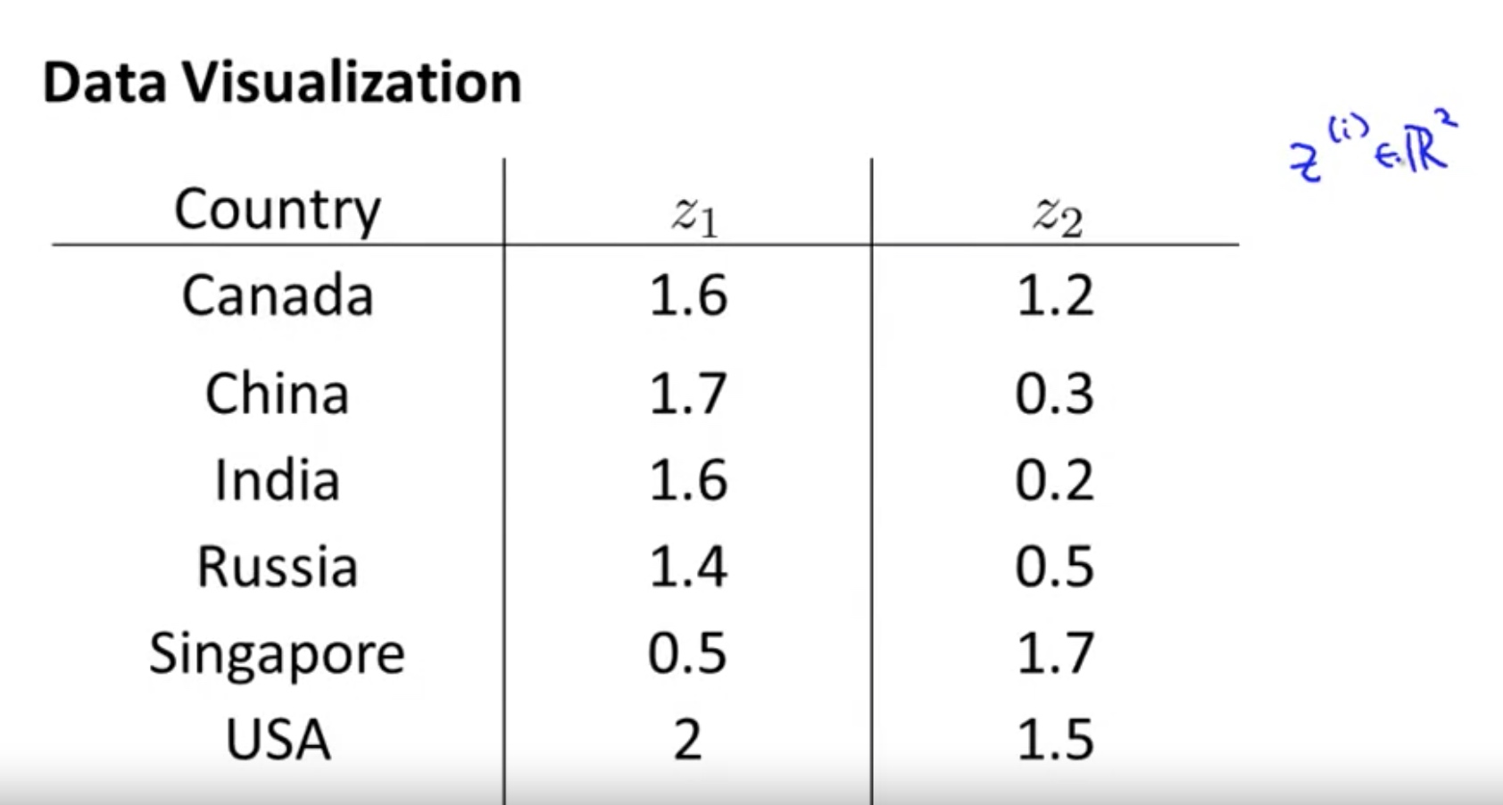
But what is the meaning of these new features? -> it is a difficult to explain.
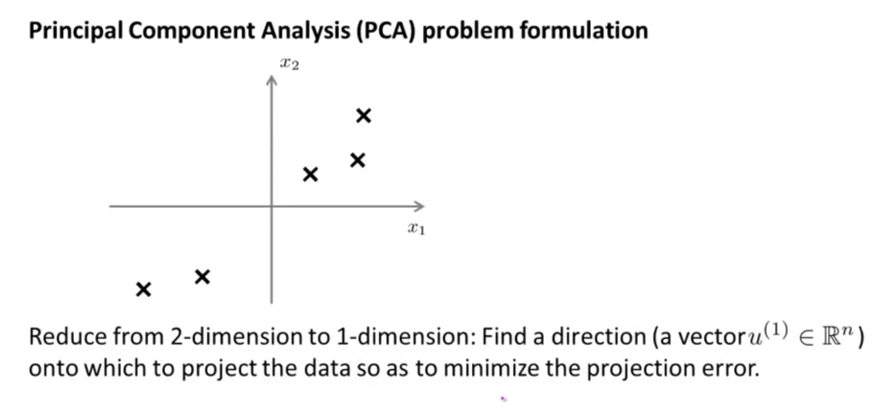
Principle Component Analysis
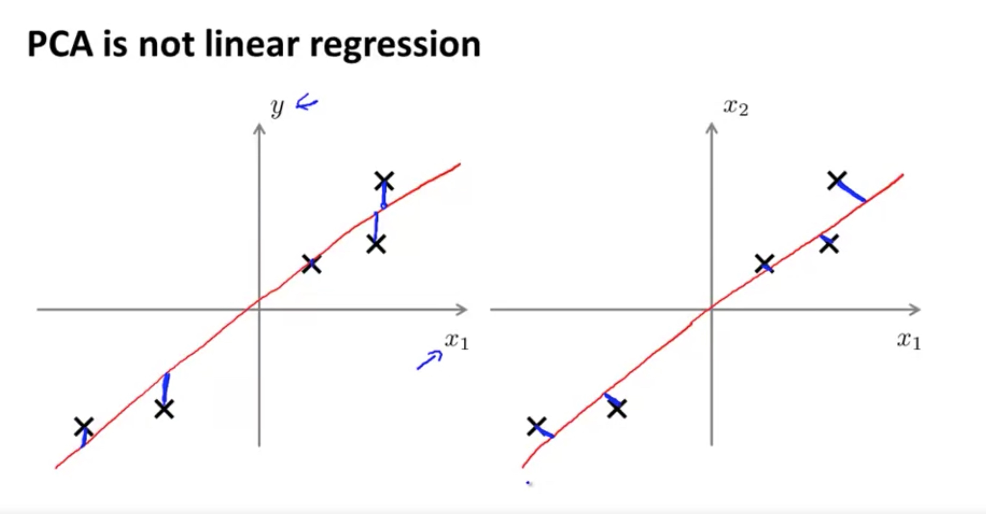
For the linear regression: $min ||Ax-y||^2$ since $Ax=(a1,a2,…,a_n)x$, the linear regression is essentially the projection of y onto the linear space of column vectors of A.
For the PCA, the first principle component is the one that: $\max ||A\mu||^2 $
Mathematically, for the linear regression, it is a problem of project a point in $R^m $ into the linear space of ${x_0,x_1,…,x_n}$. In other words, the base is given.
for the PCA, however, it is a problem of find a sub-space for the data given, so that most of the information can be maintained. In other words, the task is to find the base of the sub-space. ($\mu_1, …, \mu_k \in R^n$)
Details in Mathematics
First Component
In order to maximize variance, the first weight vector w(1) thus has to satisfy:
\[\begin{equation} \mathbf{w}_{(1)}=\underset{\|\mathbf{w}\|=1}{\arg \max }\left\{\sum_{i}\left(t_{1}\right)_{(i)}^{2}\right\}=\underset{\|\mathbf{w}\|=1}{\arg \max }\left\{\sum_{i}\left(\mathbf{x}_{(i)} \cdot \mathbf{w}\right)^{2}\right\} \end{equation}\]Equivalently, writing this in matrix form gives
\[{\displaystyle \mathbf {w} _{(1)}={\underset {\Vert \mathbf {w} \Vert =1}{\operatorname {\arg \,max} }}\,\{\Vert \mathbf {Xw} \Vert ^{2}\}={\underset {\Vert \mathbf {w} \Vert =1}{\operatorname {\arg \,max} }}\,\left\{\mathbf {w} ^{T}\mathbf {X^{T}} \mathbf {Xw} \right\}}\]Since $w_{(1)}$ has been defined to be a unit vector, it equivalently also satisfies
\[{\displaystyle \mathbf {w} _{(1)}={\underset {\Vert \mathbf {w} \Vert =1}{\operatorname {\arg \,max} }}\,\{\Vert \mathbf {Xw} \Vert ^{2}\}={\underset {\Vert \mathbf {w} \Vert =1}{\operatorname {\arg \,max} }}\,\left\{\mathbf {w} ^{T}\mathbf {X^{T}} \mathbf {Xw} \right\}}\]The quantity to be maximised can be recognised as a Rayleigh quotient. A standard result for a positive semidefinite matrix such as $X^TX$ is that the quotient’s maximum possible value is the largest eigenvalue of the matrix, which occurs when w is the corresponding eigenvector.
With $w_{(1)}$ found, the first principal component of a data vector $x_{(i)}$ can then be given as a score $t_{1(i)} = x_{(i)} ⋅ w_{(1)}$ in the transformed co-ordinates, or as the corresponding vector in the original variables $t_{1(i)}w_{(1)} = <x_{(i)} * w_{(1)}>w_{(1)}$
Further Component
The kth component can be found by subtracting the first k − 1 principal components from X:
\[\begin{equation} \hat{\mathbf{X}}_{k}=\mathbf{X}-\sum_{s=1}^{k-1} \mathbf{X} \mathbf{w}_{(s)} \mathbf{w}_{(s)}^{\mathrm{T}} \end{equation}\]and then finding the weight vector which extracts the maximum variance from this new data matrix
\[\begin{equation} \mathbf{w}_{(k)}=\underset{\|\mathbf{w}\|=1}{\arg \max }\left\{\left\|\hat{\mathbf{X}}_{k} \mathbf{w}\right\|^{2}\right\}=\arg \max \left\{\frac{\mathbf{w}^{T} \hat{\mathbf{X}}_{k}^{T} \hat{\mathbf{X}}_{k} \mathbf{w}}{\mathbf{w}^{T} \mathbf{w}}\right\} \end{equation}\]It turns out that this gives the remaining eigenvectors of $X^TX$, with the maximum values for the quantity in brackets given by their corresponding eigenvalues. Thus the weight vectors are eigenvectors of $X^TX$. The full principal components decomposition of X can therefore be given as $\mathbf{T} = \mathbf{X} \mathbf{W}$ where W is a p-by-p matrix of weights whose columns are the eigenvectors of $X^TX$. The transpose of W is sometimes called the whitening or sphering transformation. Columns of W multiplied by the square root of corresponding eigenvalues, i.e. eigenvectors scaled up by the variances, are called loadings in PCA or in Factor analysis.
PCA algorithm
Step 1: Data Preprocessing Mean Normalization, so that the features centers in the original point. Feature scaling is necessary;
\[X=\frac{[X-mean(X)]}{std(X)}\]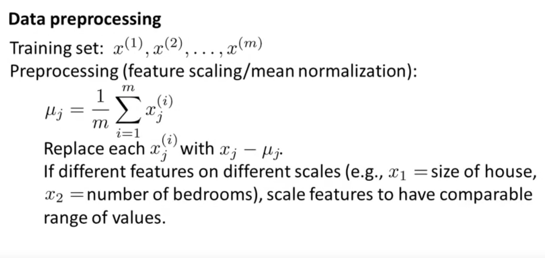

Vectorization:
Mean normalization and optionally feature scaling:
\[X= \text{bsxfun}(@minus, X, mean(X,1))\] \[\sum =\frac{1}{m} X^TX\] \[[U,S,V]=svd(\sum )\]Then we have:
\[U=\left[\begin{array}{cccc}{|} & {|} & {} & {|} \\ {u^{(1)}} & {u^{(2)}} & {\ldots} & {u^{(n)}} \\ {|} & {|} & {} & {|}\end{array}\right] \in \mathbb{R}^{n \times n}\]$x\in R^n \to z\in R^k: $
$\text{Ureduce}=U(~: ~, 1:k)$
$z=\text{Ureduce}^T*X$
Note 1: $x_0^{i} \neq 0$ for this convention. Note 2: $U$ is from $USV^*=X^TX$, therefore U is $R^{n\times n}$. It is the eigenvector of X.
Applying PCA
Reconstruction from compressed representation
\[z=\text{Ureduce}^T*X \Longrightarrow X_{Approx}=\text{Ureduce}*z\]here $ X_{Approx } \in R^n $
Choose the number of principle component

Since S is the eigenvalues for $X^TX$, $s_ii$ is actually the square of $s_i$, which is the eigenvalue for X.
\[\begin{array}{l}{\text { Choosing } k \text { (number of principal components) }} \\ {[\mathrm{U}, \mathrm{S}, \mathrm{V}]=\mathrm{svd}(\text { Sigma })} \\ {\text { Pick smallest value of } k \text { for which }} \\ {\qquad \frac{\sum_{i=1}^{k} S_{i i}}{\sum_{i=1}^{m} S_{i i}} \geq 0.99} \\ {\text { (99% of variance retained) }}\end{array}\]Advice for applying PCA
Supervised learning speedup
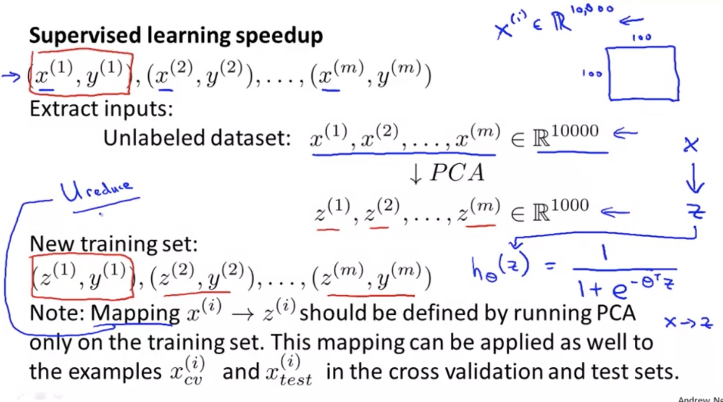
Note: must normalize the X before PCA. feature scaling is optional but recommended if large variance among features.
The same transformation must be done for $x_{val}$ and $x_{test}$
In summary, application for PCA:
- Compression
- Reduce memory/disk needed for storage of data
- speed up learning algorithm
- Visualization
Note: It might work ok, but it is generally a bad application to use PCA to prevent overfitting. Use regularization instead
\[\min _{\theta} \frac{1}{2 m} \sum_{i=1}^{m}\left(h_{\theta}\left(x^{(i)}\right)-y^{(i)}\right)^{2}+\frac{\lambda}{2 m} \sum_{j=1}^{n} \theta_{j}^{2}\]If the overfitting is the problem, utilization of PCA would probably throw away some useful information.
People like to utilized PCA for any ML problem:
\[\begin{array}{l}{\text { Design of ML system: }} \\ {\text { - Get training set }\left\{\left(x^{(1)}, y^{(1)}\right),\left(x^{(2)}, y^{(2)}\right), \ldots,\left(x^{(m)}, y^{(m)}\right)\right\}} \\ {\left.\left. \text { - Run PCA to reduce } x^{(i)} \text { in dimension to get } z^{(i)} \right)\right\}} \\ {\text { - Train logistic regression on }\left\{\left(z^{(1)}, y^{(1)}\right), \ldots,\left(z^{(m)}, y^{(m)}\right)\right\}} \\ {\text { - Test on test set: Map } x_{t e s t}^{(i)} \text { to } z_{test}^{(i)} . \text { Run } h_{\theta}(z) \text { on }} \\ {\quad\left\{\left(z_{t e s t}^{(1)}, y_{t e s t}^{(1)}\right), \ldots,\left(z_{t e s t}^{(m)}, y_{t e s t}^{(m)}\right)\right\}}\end{array}\]Before implementing PCA, it is better to try running without the PCA with the original/raw data. Only if it does not do what is desired, then implement PCA.
Anomaly Detection
Density Estimation
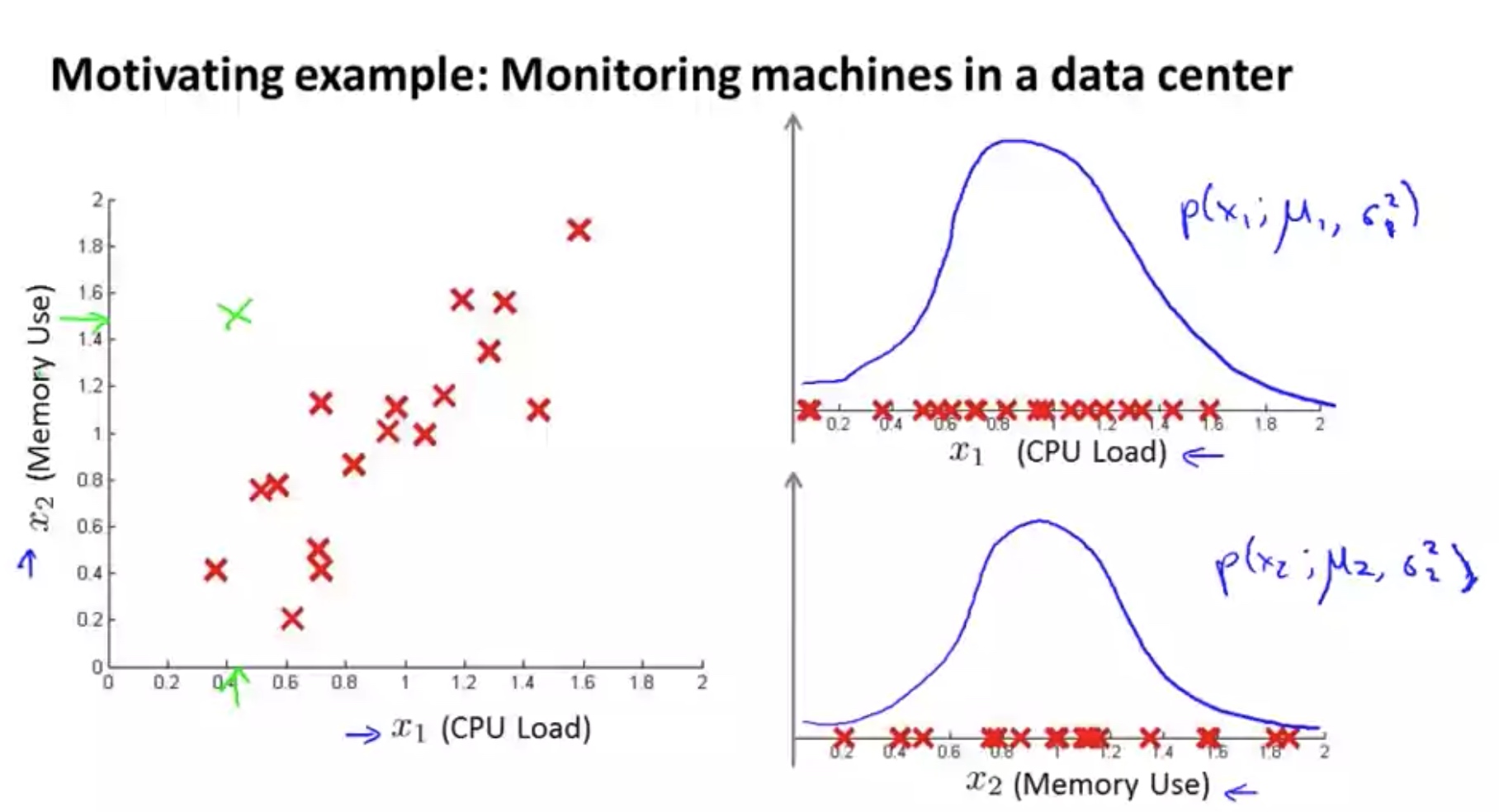
Problem Motivation
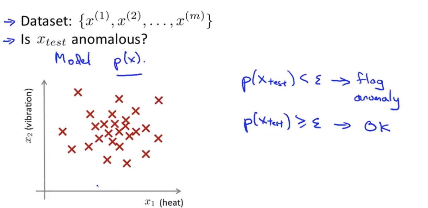

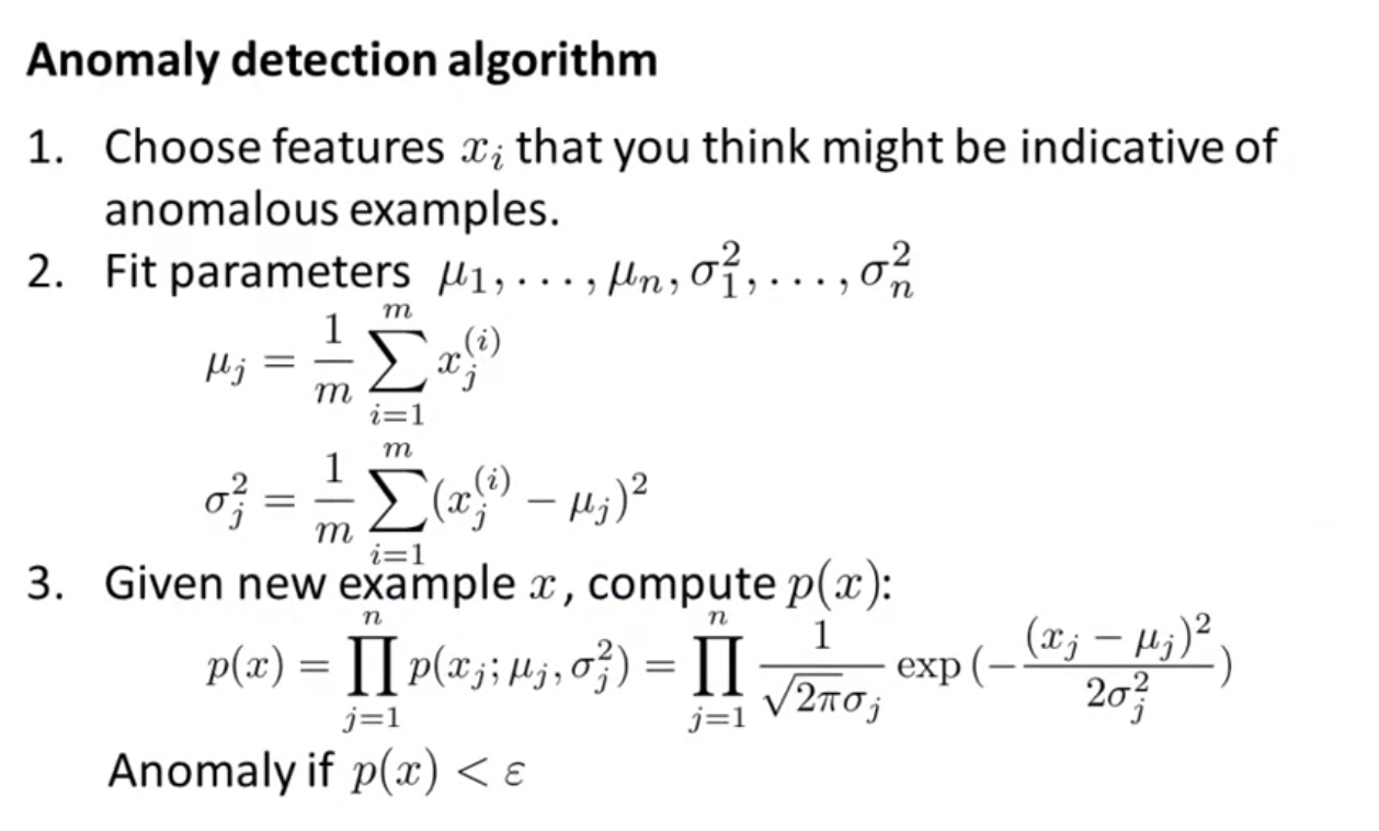
Algorithm for a Anomaly detection
Building Anomaly Detection System
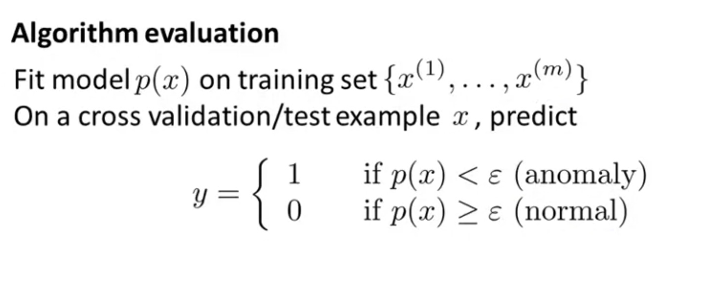
Due to possible skewness of the data or label, the accuracy of prediction is not a good measure of the performance of algorithm.
- Possible evaluation metrics:
Precision:
\[\frac{\# True ~Positives}{\#~ Total~Predicted~Positives}\]Recall:
\[\frac{\# True ~Positives}{\#~ Total~Actual~Positives}\]
$F_1 ~ Score=2 \frac{PR}{P+R}$
- Use cross validation set to choose parameter $\epsilon $
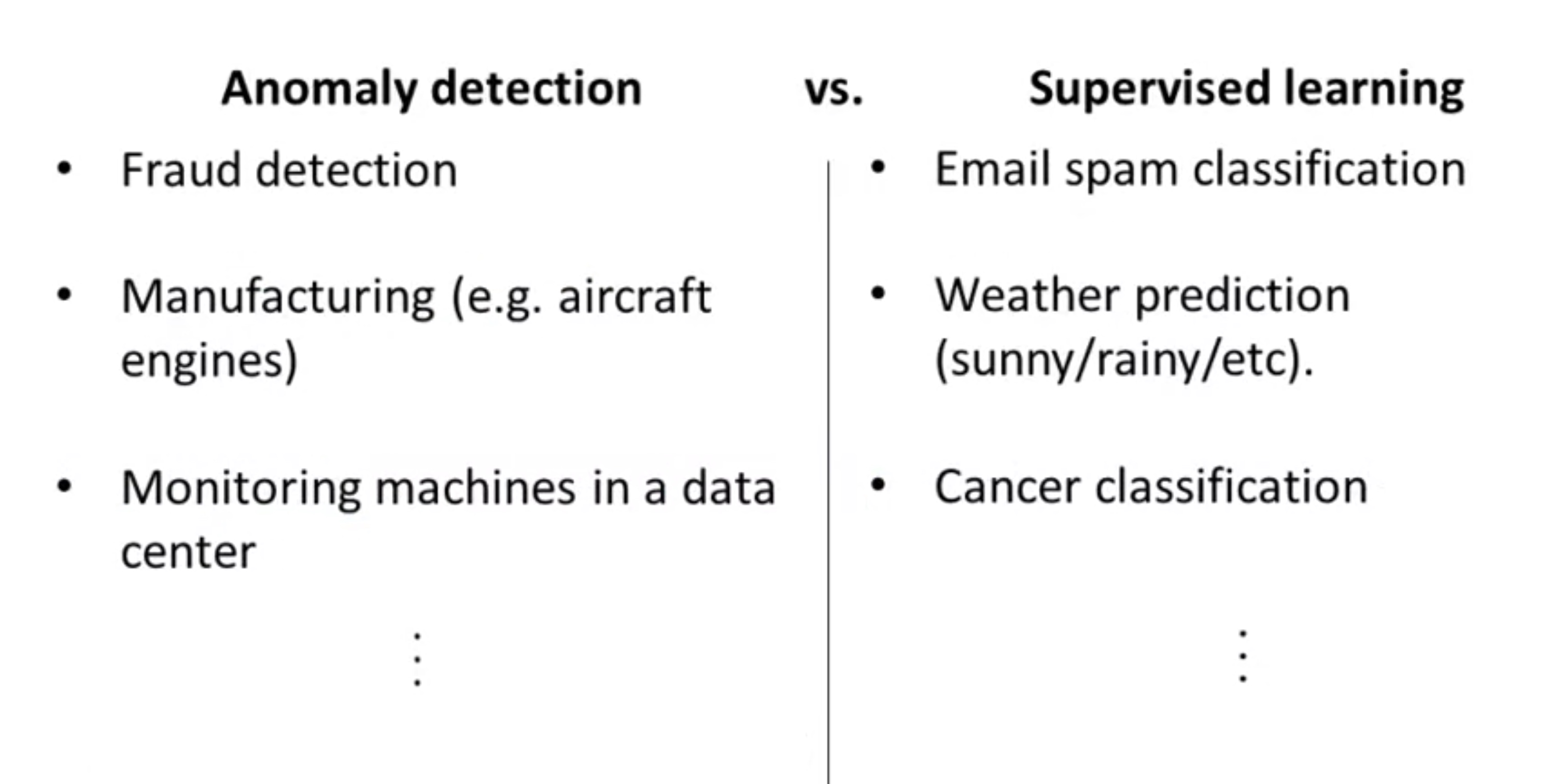
Anomaly Detection (Gaussian) VS. Supervised Learning
Since we have labeled data, why not just use supervised learning to detect to anomaly?
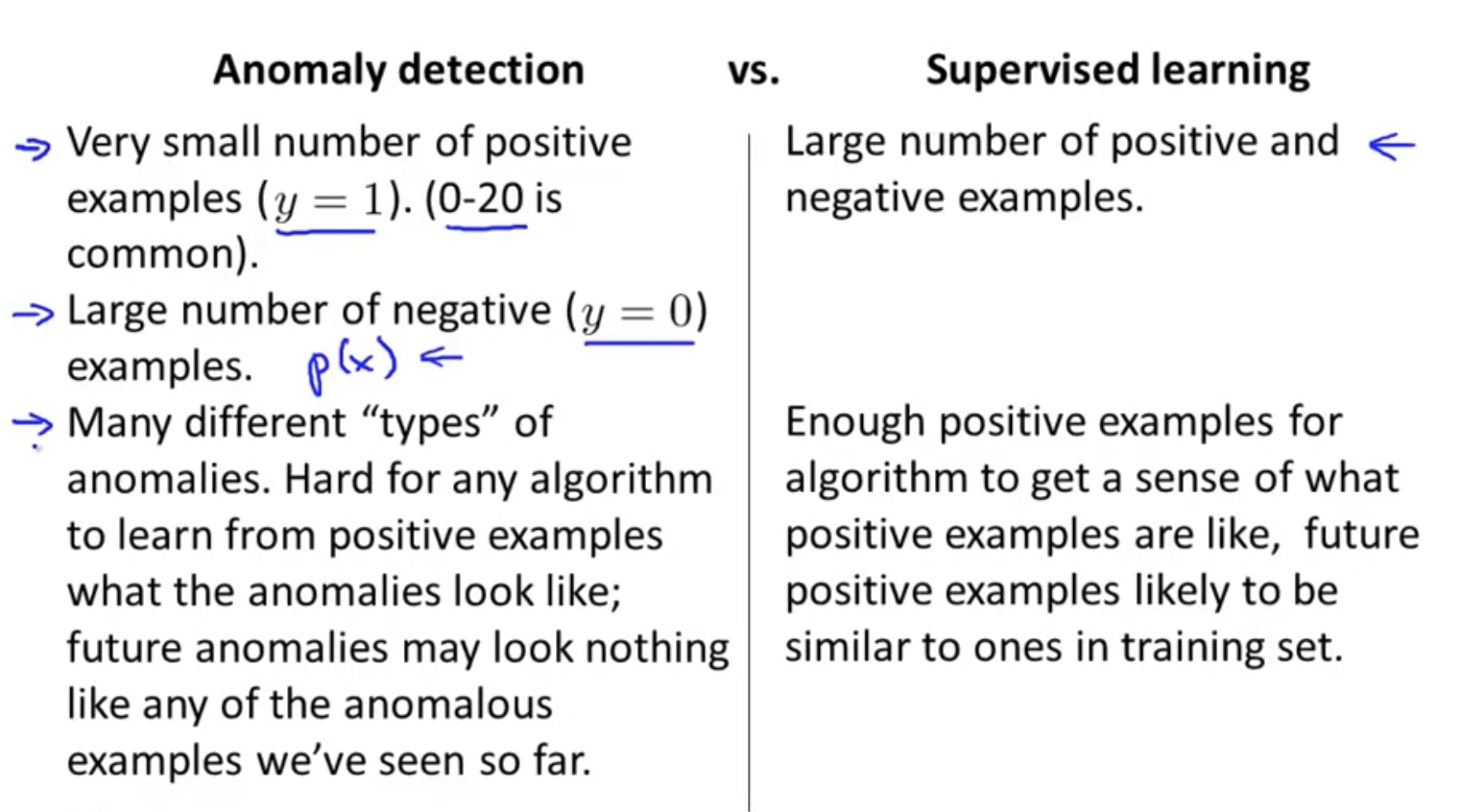
Few features: use anomaly detection, as the limited number of features make it hard to learn.
Choosing What Features to Use in the Anomaly Detection
- If the feature is Non-Gaussian, it is better to transform the feature to be more like Gaussian distribution
- If it is difficult to identify the anomaly with the current features, it will helpful if more features can be added, specially based on observation of anomaly.
Multivariant Gaussian Distribution
In the previous anomaly detection algorithm, the features are assumed to be independent and normally distributed. If we want to consider the dependency or correlation among the n features, we can use multivariant gaussian distribution.
Note: use PCA to capture the normal?
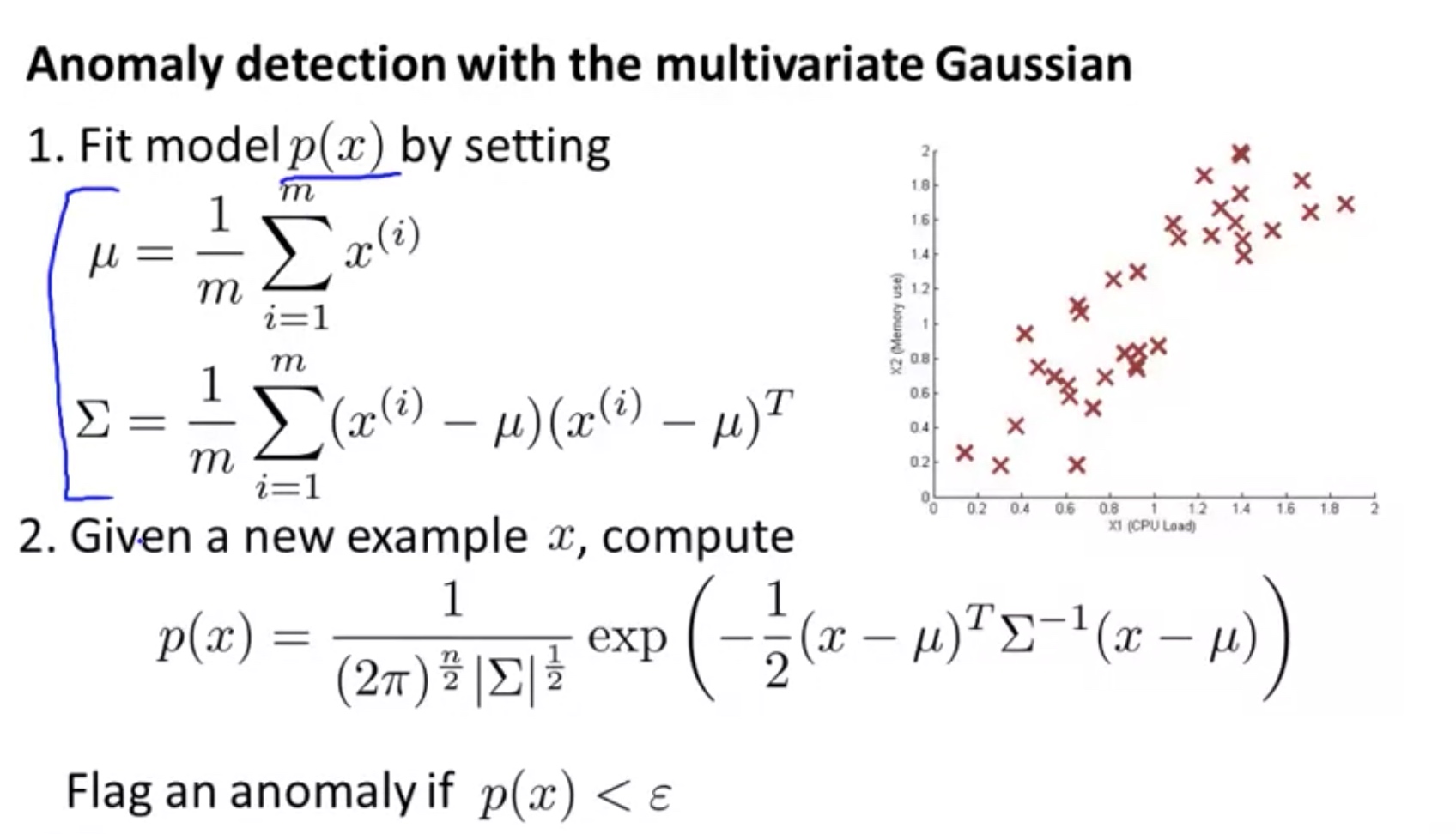
\[\begin{array}{l}{\text { Multivariate Gaussian (Normal) distribution }} \\ {x \in \mathbb{R}^{n} . \text { Don't model } p\left(x_{1}\right), p\left(x_{2}\right), \ldots, \text { etc. separately. }} \\ {\text { Model } p(x) \text { all in one go. }} \\ {\text { Parameters: } \mu \in \mathbb{R}^{n}, \Sigma \in \mathbb{R}^{n \times n} \text { (covariance matrix) }}\end{array}\] \[{\displaystyle f_{\mathbf {X} }(x_{1},\ldots ,x_{k})={\frac {\exp \left(-{\frac {1}{2}}({\mathbf {x} }-{\boldsymbol {\mu }})^{\mathrm {T} }{\boldsymbol {\Sigma }}^{-1}({\mathbf {x} }-{\boldsymbol {\mu }})\right)}{\sqrt {(2\pi )^{k}|{\boldsymbol {\Sigma }}|}}}}\] \[\begin{array}{l}{\text { Parameters } \mu, \Sigma} \\ {\qquad p(x ; \mu, \Sigma)=\frac{1}{(2 \pi)^{\frac{n}{2}}|\Sigma|^{\frac{1}{2}}} \exp \left(-\frac{1}{2}(x-\mu)^{T} \Sigma^{-1}(x-\mu)\right)}\end{array}\]- Parameter Filtering: Given training set ${x^{(1)}, x^{(2)}, \ldots, x^{(m)} }$, we can calculate the parameters:
here $\mu , x^{(i)} \in R^n$, in other words: $\sum =E(X-\mu)^T (X-\mu)$ here $X=[{x^{(1)}}’;{x^{(2)}}’;…;{x^{(m)}}’]$ therefore we have: $X’=[{x^{(1)}},{x^{(2)}},…,{x^{(m)}}]$
- Algorithm:
Note that for the multivariate gaussion:
- the n features $\in R^m$ must be linearly independent, i.e. full rank of n:==> must have m$\geq$n, otherwise we have some $x^T \sum x=0$ which means $\sum $ is non-invertible.
- Computationally more expensive
Comments